A Novel Hybrid Classification Model - LightGBM With Neural Net
1 Introduction
This project is made for a competition, which I received grand prize. The key objective of this challenge is to build a machine learning model that handles given data set, with the most suitable encoding schemes and the least set of feature variables. Also, it requires no correlated variables in the set of predictors. The model should be built based on the Challenge dataset, and to predict the observations in Evaluation dataset.
Here is a data sample for Challenge dataset.

2 Data Evaluation
The received datasets files are “Challenge Data Set.xlsx” (called Challenge dataset) and “Evaluation Data Set.xlsx” (called Evaluation dataset).
In the Challenge dataset, there are 3000 records with 31 variables. Among those variables, only one variable with label “XC”, is categorical with 5 levels – “A”, “B”, “C”, “D” and “E”, and the rest are numerical variables. For the binary response “y”, its mean is 0.31, so the class 0 and 1 is unbalanced. Also, there are 7000 records in the Evaluation dataset. For both of the datasets, there are no missing values.
Furthermore, in terms of the variable “XC”, you can find the distribution of 5 levels in Evaluation dataset, and Challenge dataset in Table 1, as well as the distribution of response “y” grouped by those levels.
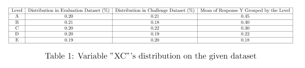 From the table, you can see the 5 levels are nearly evenly distributed in both datasets. Later, We will transform this categorical variable by replacing each level with their related the average of response “y”.
3 Method
3.1 Motivation
For this project, we proposed a novel hybrid model, which is a combination of neural network and LightGBM (NN +lightGBM). Here are my motivations on combining those two models
Comparing with other widely used machine learning models, lightGBM has its own unique advantages for this classification assignment. First, as a Gradient Boosting Decision Tree (GBDT) method, it is very convenient to apply lightGBM to demonstrate the importance of features. Meanwhile, unlike other GBDT algorithms, such as XGboost, lightGBM can deal with categorical data. It gives me more flexibility on dealing with categorical variables. Also, lightGBM is better in training speed and space efficiency than other GBDT algorithms. Furthermore, unlike some traditional machine learning methods, lightGBM can handle data with imbalanced classes
For this supervised learning , neural networks can be used to perform feature learning, since they learn a representation of their input at the hidden layer(s) which is subsequently used for classification at the output layer. The later experiments show by adopting those newly extracted features, the model’s performance increases significantly.
Overall, the instability of the single model prediction and the shallow model’s unsatisfactory data feature mining inspired me to move toward deep learning and ensemble learning. Hence, we decided to adopt this fusion model. This model has shown promising performance in terms of the F1 score.
3.2 Pipeline Details
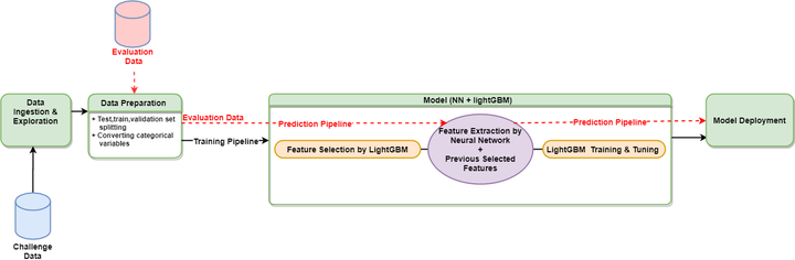
The model pipeline can be divided into three parts
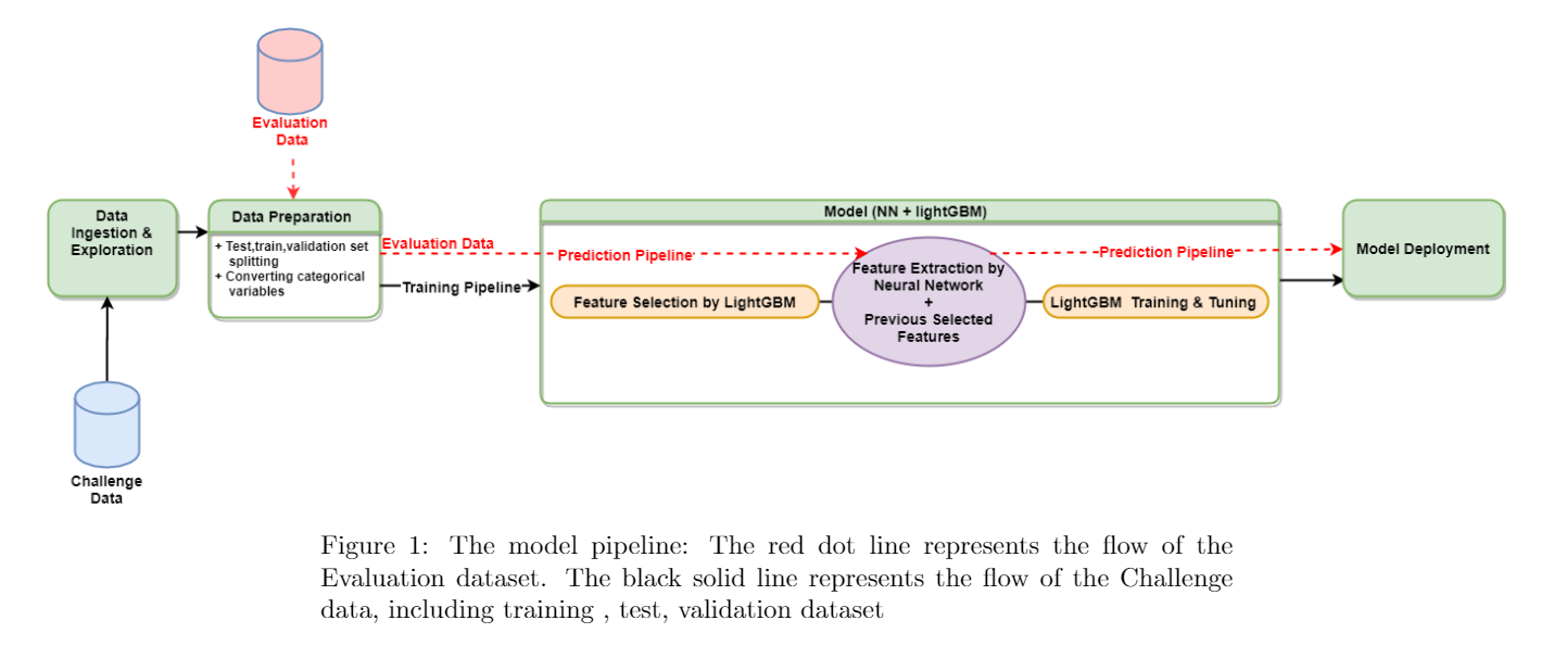
3.2.1 Data Preparation (CleanData.py)
In this part, the data is divided into test, training and validation set randomly with ratio, 2:6:2. Meanwhile, all sets’ variable “XC” is transformed into numerical type, by replacing that level with the average of “Y” under that level in the training set. This transformation will be applied to all sets, including the Evaluation dataset.
3.2.2 Model (Model.py)
This part has 3 steps.
Step 1-Feature Selection by lightGBM: The goal is to limit the number of features used in the final model based on features’ importance and correlation with others. The averaged importance score for each feature was calculated by using lightGBM . Next, we calculate the correlation within those features. Then, I select features which have high importance scores (higher than an importance score threshold) and low correlation (lower than a correlation threshold). For the features which are highly correlated, the one with highest importance score will be chosen from correlated features sets. The feature selection is done in the training set.
Step 2- Exact features by neural networks:After obtaining important features, this pipeline will generate new features from those selected features, by extracting the last hidden layers from a neural network built on a training set. The hyperparameters of this neural network were tuned by grid-searching in the validation set. Finally, the training, test, validation and Evaluation set will be transformed with the last hidden layers to get new features. Notice all observations from all sets are normalized based on the training set.
Step 3- LightGBM tuning and testing:After combining selected features and extracted features from step 1 and 2, the transformed training and validation data will be used for training and hyperparameter tuning. The tuned model will be saved for later deployment.
The overall operations on the Evaluation data:
- Dropping the unimportant features in step 1, and keep the set of selected features, S1
- Normalizing S1 by the std and mean of the training set, call it S2
- Extracting hyper features from S2 by the neural network trained in step2, call it S3
- Combining S1 and S3 to get the final feature set, S4
- Using the trained lightGBM to predict the Evaluation dataset’s labels based on S4.
3.2.3 Model Deployment (Wrapper.py)
The pipeline will load the saved model to predict the label for the transformed Evaluation dataset.
3.3 Model Details
Features’ Importance Score: In lightGBM, The importance of a feature is the number of times the feature is used in a model. In terms of feature importance score, the train set is divided into several folds. In each fold, we calculate the feature importance for each feature, and average the importance for each feature over all folds. The averaged result will be the feature importance score. The logic behind this is using randomness in each run of lightGBM fitting. Therefore, the ensemble mean can be strong evidence to reflect the importance of features. Here is the feature importance graph.
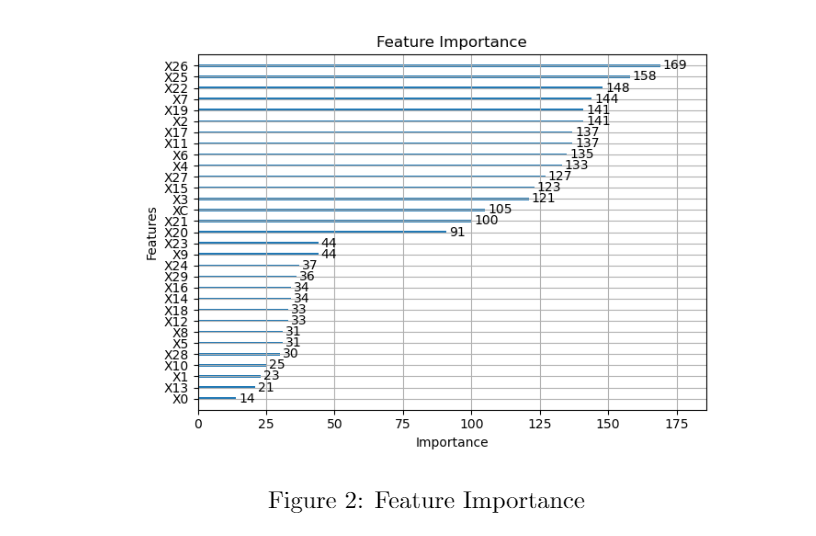
As the figure shows, there is a big jump in the feature importance score between “X20” and “X23”. Hence, features can be easily grouped into two sets based on importance score. This indicates how important the feature is and how to control the number of features when building the model.
Neural Networks:This neural network has 5 layers- one input layer, two dense hidden layers, one output layer and there is a drop-out layer to avoid over-fitting. Figure 3 shows the final selected neural network’s structure.
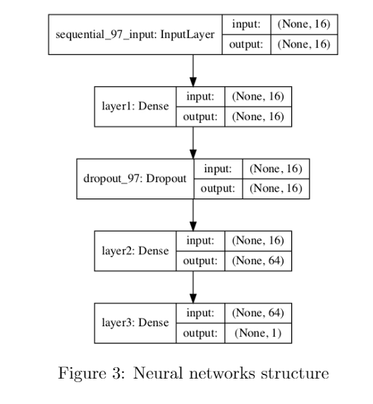
The hyperparameters of the NN include the size of the neurons, the activation function and the drop-out rates. The output layer uses sigmoid function, thus for each sample, it predicts a value between 0 to 1 – the probability that this sample belongs to class 1.
4 Performance
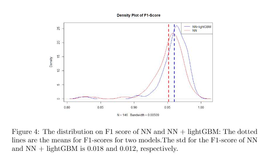
For testing purposes, we run the model for 146 times. For getting a convincing result, in each run, the pipeline will randomly split the training, test, and validation dataset. Also, for all models’ hyperparameters and feature sets will be refitted, and reselected. As a comparison to NN+lightGBM, the prediction results from the neural network, which used to generate features, were also recorded. Figure 4 shows the distribution of the F1 score from all runs. Both model’s averaged F1-scores are above 0.95, but NN+lightGBM has better performance overall and has a lower standard deviation in F1-scores. Thus NN+lightGBM is a more robust model compared to NN. It also means if you are willing to sacrifice some F1-score, you can use the trained neural network to predict for gaining some efficiency.
In terms of dealing with imbalance class, ROC curves may present an overly optimistic view of an algorithm’s performance if there is a large skew in the class distribution. However, Precision-Recall (PR) curves, often used in Information Retrieval , have been cited as an alternative to ROC curves for tasks with a large skew in the class distribution.
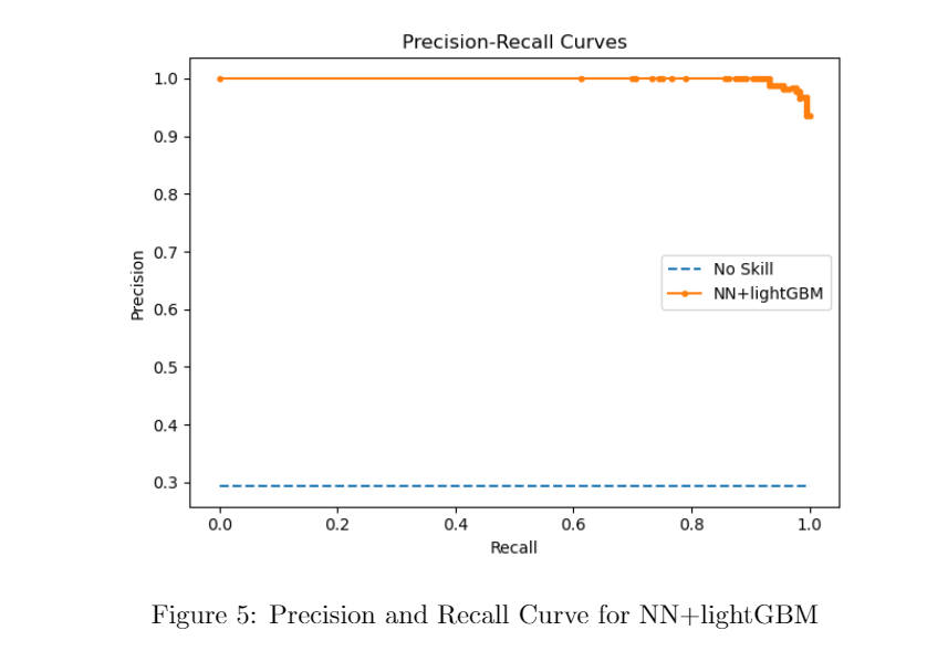
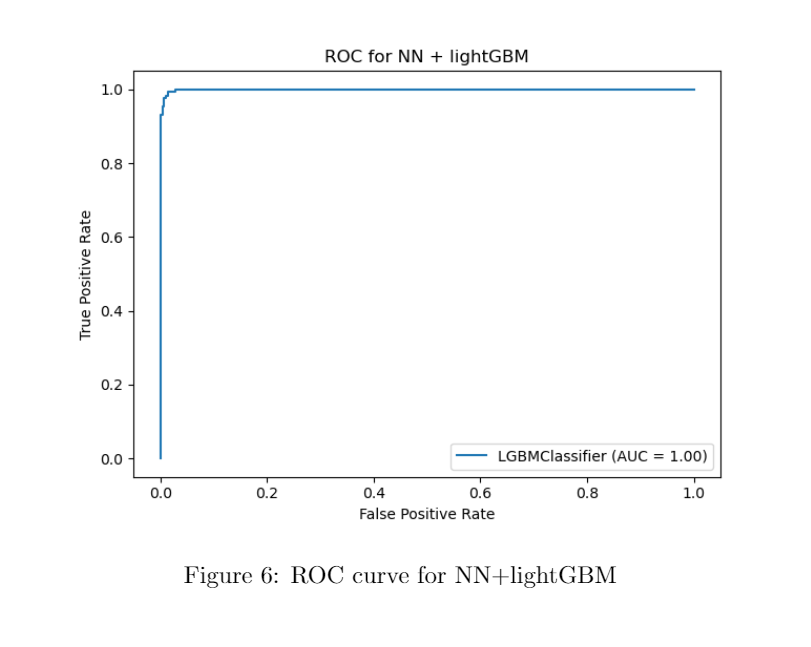 Here is the precision and recall curve on one run. The area under the curve gets to 0.998. Therefore, the model performs extremely well under the imbalance situation. we also attached a ROC curve as a comparison. In terms of limitation of the model, there is a potential risk to have overfitting, since we are using neural network and lightGBM. Also, it is hard to interpret the newly extracted features by the neural networks.
5 Code
The related code can be found from here
6 Reference
- Maura E Stokes, Charles S Davis, and Gary G Koch.Categorical dataanalysis using SAS. SAS institute, 2012.
- Guolin Ke, Qi Meng, Thomas Finley, Taifeng Wang, Wei Chen, Weidong Ma,Qiwei Ye, and Tie-Yan Liu. Lightgbm: A highly efficient gradient boostingdecision tree. In I. Guyon, U. V. Luxburg, S. Bengio, H. Wallach, R. Fergus,S. Vishwanathan, and R. Garnett, editors,Advances in Neural InformationProcessing Systems 30, pages 3146–3154. Curran Associates, Inc., 2017.
- Juliaflower. Feature selection lgbm with python, Dec 2018.
- Jason Brownlee. Roc curves and precision-recall curves for imbalanced clas-sification, Jan 2020.