How To Build Your Own Neural Net From The Scratch
1 Introduction
In this post, I will try to write a Neural Network with stochastic gradient decent (SGD) in the R, and train the Neural Network on the MNIST data set for digit recognition and report my test error (i.e. the proportion of test cases that are mis-classified). Now, let’s go over each part of my neural net.
2 About Data
The MNIST data was split into 60,000 training images, and 10,000 test images. That’s the official MNIST description. Actually, we’re going to split the data a little differently. We’ll leave the test images as is, but split the 60,000-image MNIST training set into two parts: a set of 50,000 images, which we’ll use to train our neural network, and a separate 10,000 image validation set.
Let’s write the function first for loading the data into R:
## Load the MNIST digit recognition dataset into R
## http://yann.lecun.com/exdb/mnist/
## assume you have all 4 files and gunzip'd them
## creates train$n, train$x, train$y  and test$n, test$x, test$y
## e.g. train$x is a 60000 x 784 matrix, each row is one digit (28x28)
## call:  show_digit(train$x[5,])   to see a digit.
## this code was written by:
## brendan o'connor - gist.github.com/39760 - anyall.org

load_mnist <- function() {
  load_image_file <- function(filename) {
    ret = list()
    f = file(filename,'rb')
    readBin(f,'integer',n=1,size=4,endian='big')
    ret$n = readBin(f,'integer',n=1,size=4,endian='big')
    nrow = readBin(f,'integer',n=1,size=4,endian='big')
    ncol = readBin(f,'integer',n=1,size=4,endian='big')
    x = readBin(f,'integer',n=ret$n*nrow*ncol,size=1,signed=F)
    ret$x = matrix(x, ncol=nrow*ncol, byrow=T)
    close(f)
    ret
  }
  load_label_file <- function(filename) {
    f = file(filename,'rb')
    readBin(f,'integer',n=1,size=4,endian='big')
    n = readBin(f,'integer',n=1,size=4,endian='big')
    y = readBin(f,'integer',n=n,size=1,signed=F)
    close(f)
    y
  }
  train <<- load_image_file('D:/newsite/My_Website/static/data/train-images-idx3-ubyte')
  test <<- load_image_file('D:/newsite/My_Website/static/data/t10k-images-idx3-ubyte')
  train$y <<- load_label_file('D:/newsite/My_Website/static/data/train-labels-idx1-ubyte')
  test$y <<- load_label_file('D:/newsite/My_Website/static/data/t10k-labels-idx1-ubyte')
}


show_digit <- function(arr784, col=gray(12:1/12), ...) {
  image(matrix(arr784, nrow=28)[,28:1], col=col, ...)
}
Now, we are able to load the data and show the digit
load_mnist()
str(train)  # training data
## List of 3
## $ n: int 60000
## $ x: int [1:60000, 1:784] 0 0 0 0 0 0 0 0 0 0 ...
## $ y: int [1:60000] 5 0 4 1 9 2 1 3 1 4 ...str(test) # test data## List of 3
## $ n: int 10000
## $ x: int [1:10000, 1:784] 0 0 0 0 0 0 0 0 0 0 ...
## $ y: int [1:10000] 7 2 1 0 4 1 4 9 5 9 ...show_digit(train$x[1,]) # view an image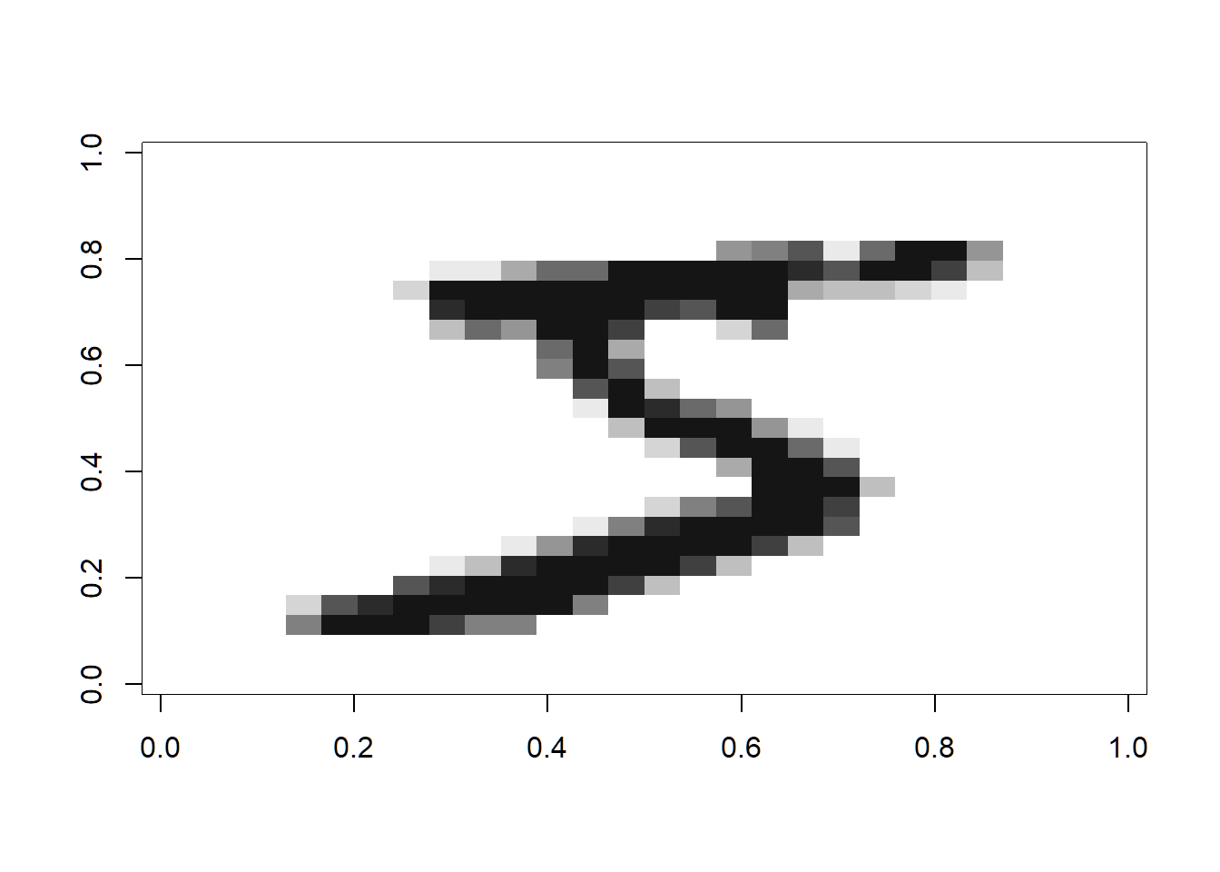
train$y[1] # the answer## [1] 53 Details of NN
Based on the functionality, I divide the code into 3 parts:
3.1 Miscellaneous
digit.to.vector(digit): The response y is a digit. we need to turn it into a vector with a 1 in the corresponding digit location. e.g. a 6 is represented as (0,0,0,0,0,0,1,0,0,0)
cost.derivative(output.activations.target, index, original.data.target): It should return derivative of squared error cost function wrt activations.
sigmoid(z)&sigmoid.prime(z): The sigmoid function and its derivative, which will be used in the backpropagation
3.2 Evaluation Funtion
evaluate(test, answer): Given an input matrix (test) and a vector (answer) of correct responses, it returns the proportion of correctly classified observations.
classify(input): Given an input vector, it returns the predicted digit.
3.3 Weights Updating
feedforard(a): Given an input a for
the network, itreturns the corresponding output. All the method does is applies the followed Equation for each layer:
\[a^{\prime}=\sigma(w a+b)\]
SGD(training.data, epochs, batch.size,eta,testing.data = NULL): It implements stochastic gradient descent
Input Parameters: MNIST training data, number of epochs, batch size, learning rate, testing.data(If “testing.data” is provided then the network will be evaluated against the test data after each epoch , and partial progress printed out. This is useful for tracking progress , but slows things down substantially)
How it work: In each epoch, it starts by randomly shuffling the training data, and then partitions it into mini-batches of the chosen size. This is an easy way of sampling randomly from the training data. Then for each mini_batch we apply a single step of gradient descent. This is done by the code
update_mini_batch, which updates the network weights and biases according to a single iteration of gradient descent, using just the training data in mini_batch.
update.mini.batch(data.x,data.y,eta,batch.size): Given a mini-batch, it applys a single step of gradient descent to each observation in the mini batch. then update the network weights and
biases.This invokes something called the backpropagation algorithm, which is a fast way of computing the gradient of the cost function.
backprop(index,data.x,data.y):Given a single observation, apply backpropagation. return the
gradient wrt biases and the gradient wrt weights.
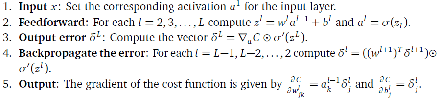
- How it work: Since we are going to talk about backpropagation, I will briefly discuss about four fundamental equations behind backpropagation. For proofs and more details, you can go check about this book Neural Networks and Deep Learning.
- An equation for the error in the output layer,\(\delta^{L}\) (BP1) \[\delta_{j}^{L}=\frac{\partial C}{\partial a_{j}^{L}} \sigma^{\prime}\left(z_{j}^{L}\right)\]
\(\partial C / \partial a_{j}^{L}\):how fast the cost is changing as a function of the jth output activation
\(\sigma^{\prime}\left(z_{j}^{L}\right)\):how fast the activation function \(\sigma\) is changing at \(z_{j}^{L}\)
- An equation for the error \(\delta^{L}\) in terms of the error in the next layer, \(\delta^{L+1}\) (BP2) \[\delta^{l}=\left(\left(w^{l+1}\right)^{T} \delta^{l+1}\right) \odot \sigma^{\prime}\left(z^{l}\right)\]
\(\left(w^{l+1}\right)^{T}\):the transpose of the weight matrix wl+1 for the \((l+1)^{th}\) layer
Notes: Suppose we know the error \(\delta^{L+1}\) at the \((l+1)^{th}\) layer. When we apply the transpose weight matrix, \(\left(w^{l+1}\right)^{T}\), we can think intuitively of this as moving the error backward through the network, giving us some sort of measure of the error at the output of the \(l^{th}\) layer. We then take the Hadamard product \(\odot \sigma^{\prime}\left(z^{l}\right)\). This moves the error backward through the activation function in layer \(l\), giving us the error \(\delta^{L}\) in the weighted input to layer \(l\).
- An equation for the rate of change of the cost with respect to any bias in the network (BP3) \[\frac{\partial C}{\partial b_{j}^{l}}=\delta_{j}^{l}\]
- An equation for the rate of change of the cost with respect to any weight in the network (BP4) \[\frac{\partial C}{\partial w_{j k}^{l}}=a_{k}^{l-1} \delta_{j}^{l}=a_{\mathrm{in}} \delta_{\mathrm{out}}\]
- \(a_{\mathrm{in}}\) is the activation of the neuron input to the weight \(w\),
- \(\delta_{\mathrm{out}}\) is the error of the neuron output from the weight \(w\).
- The algorithm: Let’s explicitly write this out in the form of an algorithm:
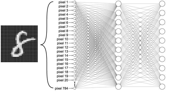
4 Parameters
For this neural net, it will have 3 layers with nodes 784,30 and 10 respectively. The step size will be 0.1 after turning. The epochs will be set as 40. Also, for simplicity, the minibatch size will be 10 intuitively.
5 Code
Let’s put those together
L <- 3 # number of layers
sizes <- c(784, 30, 10)
eta <- 0.1
epochs <- 40
batch.size <- 10
biases <- list(rnorm(sizes[2]), rnorm(sizes[3])) # layers 2 and 3
weights <- list(matrix(rnorm(sizes[2]*sizes[1]), nrow=sizes[2], ncol=sizes[1]),# layer 1 to 2
matrix(rnorm(sizes[3]*sizes[2]), nrow=sizes[3], ncol=sizes[2]))# layer 2 to 3
## w[j,k] is the weight on the link from node k to node j
## the response y is a digit. we need to turn it
## into a vector with a 1 in the corresponding digit location.
## e.g. a 6 is represented as (0,0,0,0,0,0,1,0,0,0)
## note: digit can be a vector (hence the use of sapply()).
digit.to.vector <- function(digit) {
sapply(digit, function(d) c(rep(0,d),1,rep(0,9-d)))
}
## return derivative of squared error cost function wrt activations
cost.derivative <- function(output.activations, i, data.y) {
output.activations - digit.to.vector(data.y[i])
}
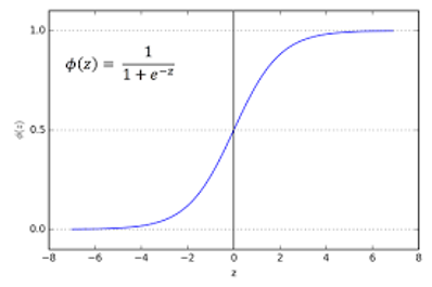
sigmoid <- function(z) 1/(1 + exp(-z))
sigmoid.prime <- function(z) sigmoid(z) * (1-sigmoid(z))
## given an input matrix (test) and a vector (answer) of correct responses,
## return the proportion of correctly classified observations.
evaluate <- function(test, answer) {
accuracy = rep(0,nrow(test))
for ( i in 1:nrow(test)){
test_results = classify(feed.forward(test[i,]))
accuracy[i]= 1*(test_results==answer[i])
}
return(mean(accuracy))
}
## given an input vector, return the predicted digit
classify <- function(input) {
test_results = which.max(input)-1
return (test_results)
}
## given an input vector a, return the vector of output activations
feed.forward <- function(a) {
for ( i in 1:(L-1 )) {
a = sigmoid(weights[[i]] %*% a + biases[[i]])}
return (a)
}
## input: MNIST training data, number of epochs, batch size, learning rate
## for each epoch:
## call update.mini.batch with a random sample of batch.size observations
## until all of the training data is used.
SGD <- function(training.data, epochs, batch.size,eta,testing.data = NULL) {
training.data.x=training.data$x
training.data.y=training.data$y
if (!is.null(testing.data)) {
testing.data.x=testing.data$x
testing.data.y=testing.data$y
n_test = nrow(testing.data.x)}
n = nrow(training.data.x)
number.batch = ceiling(n/batch.size)
for( j in 1:epochs){
rows = sample(nrow(training.data.x))
shuffle.x = training.data.x[rows,]
shuffle.y = training.data.y[rows]
index = split(seq_len(nrow(training.data.x)),rep(1:number.batch,each=batch.size))
mini_batch.x = lapply(index,function(i) shuffle.x[i,])
mini_batch.y = lapply(index,function(i) shuffle.y[i])
for(i in 1:number.batch){
update.mini.batch(mini_batch.x[[i]],mini_batch.y[[i]],eta,batch.size)
}
if (!is.null(testing.data)) {
result_test = evaluate(testing.data.x,testing.data.y)
cat("Epoch", j,":", result_test,"\n")
}
else{
cat("Epoch", j,"complete\n")
}
}
}
## given a mini-batch, apply a single step of gradient descent to each
## observation in the mini batch. then update the network weights and
## biases.
update.mini.batch <- function(data.x,data.y,eta,batch.size) {
delta.nabla.b=vector(mode = "list", length = batch.size)
delta.nabla.w=vector(mode = "list", length = batch.size)
for( i in 1: batch.size){
delta = backprop(i,data.x,data.y)
delta.nabla.b[[i]]=delta[[1]]
delta.nabla.w[[i]]=delta[[2]]
}
for ( j in 1:(L-1)){
# sum over the mini_batch
sum.b=Reduce('+',lapply(1:batch.size, function(i) delta.nabla.b[[i]][[j]]))
sum.w=Reduce('+',lapply(1:batch.size, function(i) delta.nabla.w[[i]][[j]]))
weights[[j]]<<-weights[[j]]-eta/batch.size*sum.w
biases[[j]]<<-biases[[j]]-eta/batch.size*sum.b
}
}
## given a single observation, apply backpropagation. return the
## gradient wrt biases and the gradient wrt weights.
backprop <- function(index,data.x,data.y) {
matrix.size= lapply(c(1:L), function(i) rep(0,sizes[i]))
a=matrix.size
matrix.size[[1]]= NULL
z= matrix.size
delta = matrix.size
nabla.w = weights#they are the same size, using the weights size
## feedforward
a[[1]] <- data.x[index,]
for (i in 1:(L-1)){
z[[i]]=weights[[i]] %*% a[[i]] + biases[[i]]# weighted input to hidden layer
a[[i+1]]=sigmoid(z[[i]]) # activation out of the hidden layer
}
## compute the error in the output layer
delta[[L-1]] = cost.derivative(a[[L]],index,data.y) * sigmoid.prime(z[[L-1]]) # BP1
## backpropagate the error
for ( i in (L-2):1) delta[[i]] = (t(weights[[i+1]]) %*% delta[[i+1]]) * sigmoid.prime(z[[i]]) # BP2
## compute the gradients
nabla.b = delta # BP3
for ( i in 1:(L-1)) nabla.w[[i]] = delta[[i]]%*%as.vector(a[[i]])# BP4
nabla = list(nabla.b,nabla.w)
return(nabla)
}6 Performance
Now let’s run it. It runs about 15 mins overall.
SGD(train, epochs, batch.size, eta,testing.data = test)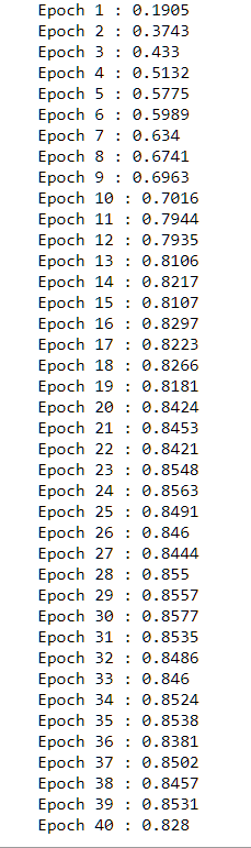
7 Reference
- Great resource to learn neural net from the beginning http://neuralnetworksanddeeplearning.com/index.html
- Course material from UMN IE 5561 Analytics and Data-Driven Decision Making