Introduction

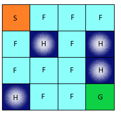
For this post, I will write my own Q-learning algorithem to solve the game from OpenAI gym called “Frozen Lake”. “Frozen Lake” is a text-based maze environment that your controller will learn to navigate. It is slippery, however, so sometimes you don’t always move where you try to go.

import gym
import numpy as np
import numpy.random as rnd
import matplotlib.pyplot as plt

%matplotlib inline
env=gym.make('FrozenLake-v0')
env.render()

[41mS[0mFFF
FHFH
FFFH
HFFG

Question

Use Q-learning to learn a policy for this problem.

About Q-Learning

Q-learning is an off policy reinforcement learning algorithm that seeks to find the best action to take given the current state. It’s considered off-policy because the q-learning function learns from actions that are outside the current policy, like taking random actions, and therefore a policy isn’t needed. More specifically, q-learning seeks to learn a policy that maximizes the total reward.

Here is the algorithm

Code

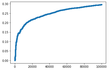
I will simulate $100,000$ episodes. Let $G^i$ be the total reward for episode $i$. In the end, I will make a plot of $\frac{1}{i}\sum_{j=1}^i G^j$ (the running average of the rewards), for $i=1$ to $100,000$. I will use a discount factor of $\gamma <1$to make it work correctly.

## initialize Q(s,a)
Q = np.zeros([env.observation_space.n,env.action_space.n])
alpha=0.8
gamma=0.95
number_episode=100000
beta=0.3
G=[]
##loop for each episode
for episode in range(number_episode):
    s=env.reset()
    G_episode=0
    done=False
    episode_length=0
    epsilon = (1/(1+episode))**(beta)
    while episode_length <=100:##  episode must be finished in 100 steps 
        if rnd.rand() < epsilon:## choose action epslone greedy
            a = env.action_space.sample()## pick a random action
        else:
            a = np.argmax(Q[s,:])##choose an action
        s_next,r,done,_=env.step(a)
        ## update Q
        Q[s,a]=Q[s,a]+alpha*(r+gamma*np.max(Q[s_next,:])-Q[s,a])
        G_episode+=r
        s=s_next
        episode_length+=1
        ## the current episode ends
        if done == True:
            break
    G.append(G_episode)
print (sum(G)/number_episode)
print (Q)    
plt.plot(np.cumsum(G)/np.arange(1,number_episode+1),'.')   

0.2956
[[5.86741698e-02 2.53313656e-01 4.24949460e-02 5.97031665e-02]
 [1.73984707e-03 1.08475750e-02 8.74301728e-03 4.87616436e-02]
 [2.90335097e-02 8.45174905e-03 8.14131382e-03 1.14581024e-02]
 [6.09104910e-04 1.03482075e-02 6.14886460e-03 1.06232220e-02]
 [2.02138540e-01 2.35482473e-02 2.12596664e-02 3.77846690e-02]
 [0.00000000e+00 0.00000000e+00 0.00000000e+00 0.00000000e+00]
 [1.14021279e-02 3.46033458e-05 2.85163045e-04 3.67230129e-06]
 [0.00000000e+00 0.00000000e+00 0.00000000e+00 0.00000000e+00]
 [1.24465789e-03 1.22092997e-02 4.15748858e-02 4.16826481e-01]
 [2.96607414e-02 1.09266566e-01 1.22155422e-02 3.67418410e-02]
 [2.56646265e-03 7.47419830e-01 4.32382306e-03 9.90243563e-04]
 [0.00000000e+00 0.00000000e+00 0.00000000e+00 0.00000000e+00]
 [0.00000000e+00 0.00000000e+00 0.00000000e+00 0.00000000e+00]
 [3.66591204e-01 1.01563327e-02 6.26778623e-01 4.58509757e-03]
 [1.04841677e-01 4.05469411e-01 9.80925785e-01 2.18991000e-01]
 [0.00000000e+00 0.00000000e+00 0.00000000e+00 0.00000000e+00]]





[<matplotlib.lines.Line2D at 0x23e77f78160>]

Result

In the graph, you can see the the reward converges to 0.3 after 100000 steps