3 mins of Machine Learning: Ada-boost

Last updated on Mar 12, 2020 R

1 Introduction
2 Adaboost Algorithm
3 R Code
4 Performance
5 Reference

1 Introduction

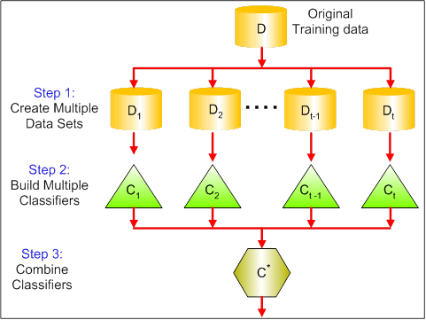
As an ensambled method, boosting refers to a general and provably effective method of producing a very accurate prediction rule by combining rough and moderately inaccurate simple predication models. It is an iterative procedure to adaptively change distribution of training data by focusing more on previously misclassified records. Initially, all N records are assigned equal weights. And unlike bagging, weights may change at the end of each boosting round. The AdaBoost algorithm, introduced in 1995 by Freund and Schapire, solved many of the practical difficulties of the earlier boosting algorithms. In this post, I will write my own Adaboost and compare its performance with other models.

2 Adaboost Algorithm

The main idea of Adaboost is to maintain a distribution or set of weights over the training set. Initially, all weights are set equally, but on each round, the weights of incorrectly classified examples are increased so that the weak learner is forced to focus on the hard examples in the training set. For more details you can check out this paper

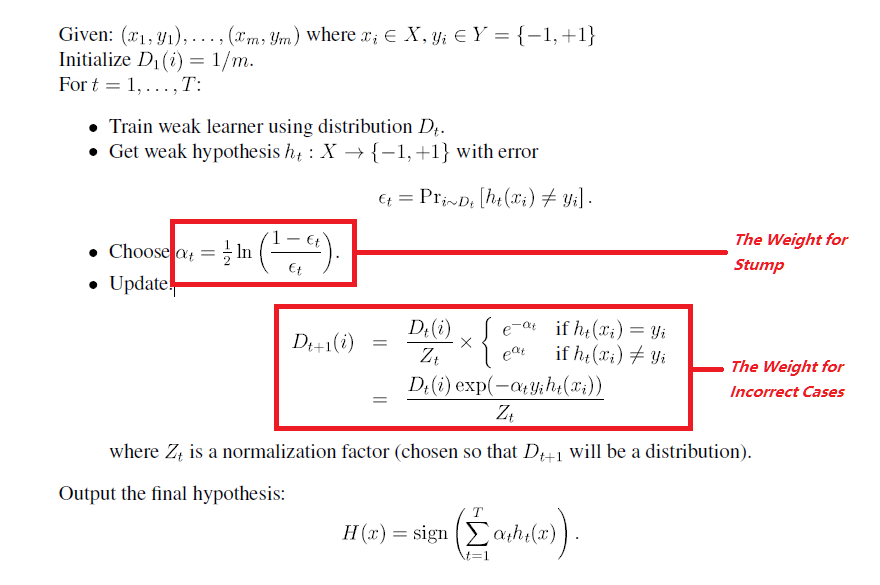
Here is the algorithm Adaboost Algorithm

3 R Code

In my code, I use regression tree with depth = 1 to be my stump

library(rpart)
## train_feature: train data's feature
## response: train data's response, it needs to be binary for my code
## test_feature: test data's feature

My_Adaboost <- function(train_feature, response, test_feature, t) {
  n = nrow(train_feature)
  m = nrow(test_feature)
  w = rep(1 / n, n)
  alpha = rep(0, t)
  result = rep(0, m)
  stump <- vector("list", t)
  
  for (i in 1:t) {
    ctrl <- rpart.control(cp = 0,
                          maxdepth = 1,
                          xval = 0)
    stump[[i]] = rpart(
      factor(response) ~ .,
      data = train_feature,
      method = "class",
      weights = w,
      control = ctrl
    )
    result_on_train = as.numeric(as.character(as.vector(
      predict(stump[[i]], train_feature, type = "class")
    )))
    epsilon = w %*% (1 * (result_on_train != response)) / sum(w)
    alpha[i] = 0.5 * (log((1 - epsilon) / epsilon))
    sign = ifelse(result_on_train == response, -1, 1)
    exp_part = exp(sign * alpha[i])
    z = w %*% exp_part
    w = (w * exp_part) / rep(z, n)
  }
  for (j in 1:t) {
    f = as.numeric(as.character(as.vector(
      predict(stump[[j]], test_feature, type = "class")
    )))
    new = alpha[j] * f
    result = new + result
  }
  pred = sign(result)
  return(pred)
}

4 Performance

## Change response
attach(stagec)
stagec= na.omit(stagec)
stagec1=stagec[,-c(1)]
stagec1$pgstat=ifelse(stagec$pgstat==0,-1,1)
head(stagec1)

##   pgstat age eet    g2 grade gleason     ploidy
## 1     -1  64   2 10.26     2       4    diploid
## 3      1  59   2  9.99     3       7    diploid
## 4      1  62   2  3.57     2       4    diploid
## 5      1  64   2 22.56     4       8 tetraploid
## 6     -1  69   1  6.14     3       7    diploid
## 9      1  73   2 11.77     3       6    diploid

##Train test data spilting
train_index=sample(c(1:nrow(stagec1)), 120)
train=stagec1[train_index,]
test=stagec1[-train_index,]
test_feature=test[,-c(1)]
train_feature=train[,-c(1)]
test_response=test[,1]
train_response=train[,1]

## Adaboost
pred=My_Adaboost(train_feature = train_feature,response = train_response,test_feature = test_feature,t=100)
mean(1*(test_response==pred))

## [1] 0.6428571

Now, let’s compare the test error to the test error from a single classification tree that is learned using rpart()

## Comparing with a single classification tree
model=rpart(factor(train_response) ~.,
      data = train_feature, method = "class")
pred_original=predict(model,test_feature,type="class")
 mean(1*(test_response==pred_original))

## [1] 0.5714286

5 Reference

Machine Learning