Let SMART be smarter

1 Introduction
Nowadays, more and more organizations start to improve their service’s quality by combing data analysis into their business decision making. The SMART learning commons(“SMART”) is one of them. As a university-sponsored academic organization, it offers UMN students some academic consulting for hundreds of classes in Walter Library, Wilson Library, Magrath Library and APARC, which is in Appleby Hall. One of the most populated services it provided is peer tutoring, which can be divided into two types, drop-ins, and appointments. With the increased usage of the SMART’s peer tutoring service, the director of the SMART realized some new conflicts between the insufficient number of tutors and the increased demand from students. Therefore, in 2017, the SMART’s director set up a survey system for collecting students’ feedbacks. In the same year, the SMART had their first-time program evaluation on their history. As a tutor of the SMART, I volunteered on implementing this program evaluation by cooperating with the director. For this evaluation, one of the main questions the director wanted to figure out was would the service type and the service time influence customers’ satisfaction score? If it would, what was the influence?
For answering those questions, the SMART’s survey’s data would be used. Since the answers of surveys are scaled from 1-5, which were discrete ordinal numbers. We decided to use ordinal logistic regression to build the model. For the ordinal logistic regression, the PSU’s online notes could be an excellent reference for understanding the statistical meanings. For the coding part, the UCLA’s tutorial offered me some specific examples on assumptions checking and coding logistic regression models on R. Furthermore, for the demonstration, we would use the function ggplot and Harvard’s article offered a specific guide on how to use it.
2 Method
2.1 Statistical Background
For ordinal logistic regression, its response will be in several ordered discrete categories. Based on the PSU’s online note, it defines: “Let the response be Y=1,2,…, J where the ordering is natural. The associated probabilities are {π1, π2,…, πJ}, and a cumulative probability of response less than equal to j is:
\[P(Y≤j)=π_1+...+π_j\]
Then a cumulative logit is defined as
\[log(\frac{P(Y≤j)}{P(Y>j)})=log(\frac{P(Y≤j)}{1-P(Y≤j)})=log(\frac{π_1+...+π_j}{π_{j+1}+⋯+π_J })\]
This logit describes the log-odds of two cumulative probabilities, one less-than, and the other greater-than type. It measures how likely the response is to be in category j or below versus in a category higher than j” (8.4 - The Proportional-Odds Cumulative Logit Model, n.d.).”
For implementing ordinal logistic regression, we should check a fundamental assumption, which is called the proportional odds assumption. It is saying that “the relationship between each pair of outcome groups is the same.” (ORDINAL LOGISTIC REGRESSION | R DATA ANALYSIS EXAMPLES, n.d.) In other words, factor’s proportions between the response in the low ranked category versus the other higher high ranked categories are the same as those, that describe the relationship between the next lowest category and all higher scores and so on. Therefore, unlike multinomial logistic regression, which its factor will have different coefficient value to match with each category, a factor of the ordinal logistic regression will have a universal odds ratio among all categories.
2.2 Data Exploration
The survey was given to students at the end of each consulting. The survey had five multiple choice questions.
*Data sample:

Those questions’ answers were all scaled by five categories, from 1-strongly disagree to 5-strongly agree. The last problem on the survey was “How satisfied are you with your experience in SMART today?”. It will be treated as the response variable to our statistical model. After almost one semester collection, 2023’s visits were recorded in total within fall 2017. During those visits, there were 747 unique students visited us. For each student, the information, such as total visits, the time for single service and the total hours for all visits, were collected. The missing data did exist, but compare to the sample size; it was safe to discard them. You could see the data sample in Appendix. Furthermore, because only drop-in service was offered in Walter Library, and the rest three locations only provided appointment based service, we could generate service type information based on the location students went to. In our model, drop-in would be labeled by 0 and appointment would be 1.
2.3 Approaches
For answering director’s question: would the service type and the service time influence people’s satisfaction rate? The response will be students’ response to the last problem, which was: “How satisfied are you with your experience in SMART today?”. Therefore, the response would have five ordered categories. My approaches were checking the proportional odds assumption first. Then, if we met the assumption, the model would have the following settings:
\[log(\frac{P(Y≤j)}{P(Y>j)})=β_0+β_1*X_(service.type)+β_2*X_(service.time) for j=1,2,3,4,5\]
If we fail to meet the assumption, the multinomial logistic regression would be used instead. The model for that would be:
\[log(\frac{P(Y=j)}{P(Y=1)})=β_0+β_1*X_(service.type)+β_2*X_(service.time) for j=1,2,3,4,5\]
3 Results
Before I started, I would like to use variable “type” to represent the service type and to use variable “hour” to represent the service hour in my result. First, I checked the proportional odds assumptions. For this project, the assumption could be understood as that, the odds ratio of “type” and “hour” that described the proportions between the lowest satisfaction score versus the other higher scores were the same as those, that described the proportions between the next lowest score and all higher scores. In other words, if I could show that, when the satisfaction score >= 2, the differences between logits for different levels of variable “type” and for different levels of variable “hour” were the same as the differences when the satisfaction score >= 3,4 and 5, then the proportional odds assumption would be likely held. For doing this, based on the UCLA’s paper’s suggestion, I break down variable “hour” temporarily into four equal-size groups. Also, I built four binary logistic models, which were models with the response classified as satisfaction rate>=2 or not, satisfaction rate>=3 or not, satisfaction rate>=4 or not and satisfaction rate>=5 or not respectively. For those models, the variables would be “type” and categorized variable “hour.” Then, I would have the coefficient for each level of each variable, which was in logit scale, for four different responses. You could find the specific coefficients in the output table.
require(foreign)
require(ggplot2)
require(MASS)
require(Hmisc)
require(reshape2)
require(readr)
f<- read_csv("D:/newsite/My_Website/static/data/smart_data.csv")

#####testing assumption
sf <- function(y) {
  c('Y>=1' = qlogis(mean(y >= 1)),
    'Y>=2' = qlogis(mean(y >= 2)),
    'Y>=3' = qlogis(mean(y >= 3)),
    'Y>=4' = qlogis(mean(y >= 4)),
    'Y>=5' = qlogis(mean(y >= 5)))
}
s <- with(f, summary(rate ~ type+hour, fun=sf))
s
## rate N= 1653
##
## +-------+-----------+----+----+--------+--------+--------+---------+
## | | |N |Y>=1|Y>=2 |Y>=3 |Y>=4 |Y>=5 |
## +-------+-----------+----+----+--------+--------+--------+---------+
## |type |No |1409|Inf |4.757176|3.670133|2.105249|0.8429082|
## | |Yes | 244|Inf |4.795791|3.522150|2.471661|1.1205912|
## +-------+-----------+----+----+--------+--------+--------+---------+
## |hour |[0.00,0.46)| 422|Inf |4.238926|3.170674|1.564612|0.5032498|
## | |[0.46,0.73)| 418|Inf |4.639572|3.362358|1.951390|0.6221954|
## | |[0.73,1.16)| 403|Inf |5.996452|4.192177|2.633752|1.2321437|
## | |[1.16,6.31]| 410|Inf |4.910201|4.394449|2.970414|1.2972147|
## +-------+-----------+----+----+--------+--------+--------+---------+
## |Overall| |1653|Inf |4.762784|3.646941|2.152978|0.8818191|
## +-------+-----------+----+----+--------+--------+--------+---------+For the better visualization of the difference between the coefficients of different levels of each variable, I generated the followed Figure from the previou Table.
plot(s, which=1:5, pch=1:5, xlab='logit', main=' ', xlim=range(s[,3:6]))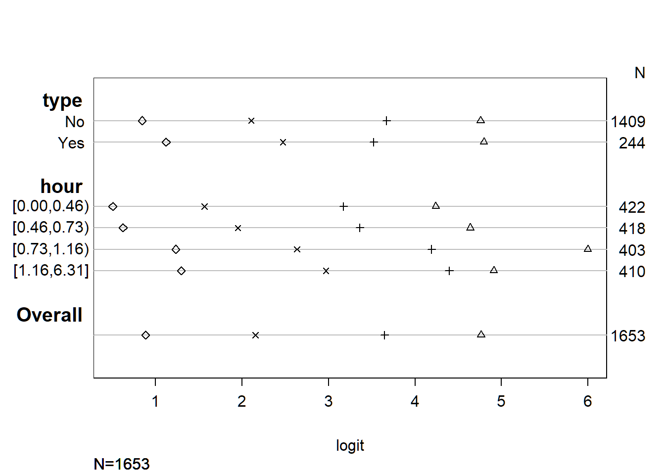
As you could see, every parameter and their levels were listed on the left side of the graph. On the right side of the chart, there listed the numbers of samples for that level. From the bottom of the graph, you could see all coefficients were in logit scale, and the number of the sample was 1653 in total. Also, there were four marks on each line. For the interpretation, let’s take variable “type” as an example. For the level “No,” from the left-hand side to the right-hand side, the first, second, third and fourth mark represented coefficients for the level “No” of variable “type” when the satisfaction score >= 2, 3, 4 and 5 respectively. For the level “Yes”, the marks, from the left to the right of the figure, represented the coefficient for the level “Yes” of variable “type” when the satisfaction score >= 2, 3, 4 and 5 respectively. What I was interested was that, if the difference between the first pair of nodes of level “Yes” and “No” was the same as that between the second, third and fourth pair of nodes in variable “type”. By comparing in this way, you could see, for variable “type”, except the third pair of nodes, the other three pairs had a similar difference between two levels. For variable “hour”, it looked like the fourth pair of nodes might have a more significant difference on coefficients than others. Therefore, it was possible that the data might not meet proportional odds assumptions.
By using polr equation from {MASS}, I built up an ordinal logistic model in R.
m <- polr(as.factor(rate) ~ type+hour, data = f, Hess=TRUE)
summary(m)
## Call:
## polr(formula = as.factor(rate) ~ type + hour, data = f, Hess = TRUE)
##
## Coefficients:
## Value Std. Error t value
## type 0.4335 0.1601 2.708
## hour 0.6096 0.1013 6.020
##
## Intercepts:
## Value Std. Error t value
## 1|2 -4.2394 0.2797 -15.1589
## 2|3 -3.1197 0.1747 -17.8608
## 3|4 -1.6125 0.1138 -14.1743
## 4|5 -0.3165 0.1004 -3.1523
##
## Residual Deviance: 2828.234
## AIC: 2840.234## view a summary of the model
summary(m)## Call:
## polr(formula = as.factor(rate) ~ type + hour, data = f, Hess = TRUE)
##
## Coefficients:
## Value Std. Error t value
## type 0.4335 0.1601 2.708
## hour 0.6096 0.1013 6.020
##
## Intercepts:
## Value Std. Error t value
## 1|2 -4.2394 0.2797 -15.1589
## 2|3 -3.1197 0.1747 -17.8608
## 3|4 -1.6125 0.1138 -14.1743
## 4|5 -0.3165 0.1004 -3.1523
##
## Residual Deviance: 2828.234
## AIC: 2840.234## store table
(ctable <- coef(summary(m)))## Value Std. Error t value
## type 0.4335141 0.1600959 2.707839
## hour 0.6095587 0.1012550 6.020037
## 1|2 -4.2393735 0.2796632 -15.158853
## 2|3 -3.1197016 0.1746679 -17.860764
## 3|4 -1.6124751 0.1137606 -14.174284
## 4|5 -0.3164977 0.1004015 -3.152320## calculate and store p values
p <- pnorm(abs(ctable[, "t value"]), lower.tail = FALSE) * 2
## combined table
(ctable <- cbind(ctable, "p value" = p))## Value Std. Error t value p value
## type 0.4335141 0.1600959 2.707839 6.772282e-03
## hour 0.6095587 0.1012550 6.020037 1.743775e-09
## 1|2 -4.2393735 0.2796632 -15.158853 6.621526e-52
## 2|3 -3.1197016 0.1746679 -17.860764 2.383528e-71
## 3|4 -1.6124751 0.1137606 -14.174284 1.321854e-45
## 4|5 -0.3164977 0.1004015 -3.152320 1.619784e-03(ci <- exp(confint(m)) )# default method gives profiled CIs## 2.5 % 97.5 %
## type 1.134097 2.126248
## hour 1.514799 2.252718## odds ratios
exp(coef(m))## type hour
## 1.542669 1.839619Therefore, for the variable “type”, by going from 0 (drop-in) to 1 (appointment), there would be an increase of 54% in the odds of giving a satisfaction score 5 versus 1,2,3 or 4 combined, given that all the other variables in the model are held constant. Then by proportional odds assumption, the odds of giving a satisfaction score of 2, 3, 4 or 5 combined versus 1 was also increased by 54% with the variable “type” change from 0 to1. On the other hand, when the variable “hour” increased 1 unit, there would be an increase of 84% in the odds of score moving from 1, 2,3 or 4 to 5. Or we can say the odds of giving 2, 3, 4 or 5 on score versus giving 1 was increased by 84% with the one unit increased on the service hour.
Once the model was generated, I could obtain predicted probabilities. You could see the probabilities plot in the follwed Figure.
newdata <- data.frame(
type = rep(0:1, 200),
hour = rep(seq(from = 0.00, to = 6.50, length.out = 100), 4))
newdata <- cbind(newdata, predict(m, newdata, type = "probs"))

##change data type from short to long
head(newdata)
## type hour 1 2 3 4 5
## 1 0 0.00000000 0.014211735 0.02809012 0.12394340 0.2552843 0.5784705
## 2 1 0.06565657 0.008898721 0.01787392 0.08369132 0.2016976 0.6878385
## 3 0 0.13131313 0.013132877 0.02604246 0.11626963 0.2466988 0.5978563
## 4 1 0.19696970 0.008219828 0.01654437 0.07807636 0.1923979 0.7047616
## 5 0 0.26262626 0.012134911 0.02413623 0.10895297 0.2378350 0.6169409
## 6 1 0.32828283 0.007592331 0.01531055 0.07278379 0.1831741 0.7211392lnewdat <- melt(newdata, id.vars = c("type", "hour"),
variable.name = "rate", value.name="Probability")
##change variable name
head(lnewdat)## type hour rate Probability
## 1 0 0.00000000 1 0.014211735
## 2 1 0.06565657 1 0.008898721
## 3 0 0.13131313 1 0.013132877
## 4 1 0.19696970 1 0.008219828
## 5 0 0.26262626 1 0.012134911
## 6 1 0.32828283 1 0.007592331names <- c(
"0"="0:drop-in",
"1"="1:appointment"
)
##plot
p=ggplot(lnewdat, aes(x =hour, y = Probability, colour = factor(rate,labels =c( "1-Very Dissatisfied","2-Dissatisfied","3-Neutral","4-Satisfied","5-Very Satisfied")))) +geom_line(size=1.5) + facet_grid(~type,labeller="label_both")+ labs(title ="The probability of giving different satisfaction score based on the service type and the length of service",subtitle="0=drop in, 1=appoinment")
p+labs(color='Satisfaction Score')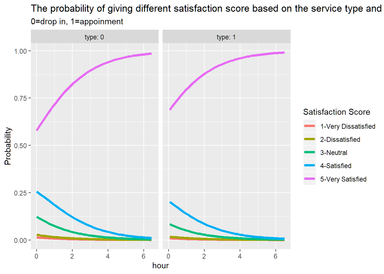
4 Conclusion
The ordinal logistic regression’s result showed that, first, students were more willing to give the highest satisfaction score 5 when they used appointment-based service, rather than the drop-in based service. Second, students were more willing to give score 5 when they receive longer service. Except score 5, the probabilities of giving out the other scores all decreased gradually. In other words, if students felt like they had already received enough attention, such as longer one-to-one service time, from their mentors, students would be more likely to score this service in 5, rather than other four scores.
For the improvement of the current model, I would suggest adding more covariates into account, such as the scores for other five questions. Since the other five questions were asked ahead, they might influence students’ decision on the survey’s last question, which was the model’s response. Furthermore, under the confidential permission was given, if mentor’s information could be included in the model, then this model would be able to offer some personal suggestions to the mentors on improving their consulting skills.
Also, I hoped this evaluation could help SMART learning commons to improve their service’s quality. The good news was that, recently, the director added a new question on their survey system, which was “Are you satisfied with the service’s time you received.” In the end, I was glad that the director took my suggestions seriously, and was willing to make more decisions based on what I found. Therefore, I believed, with more data analysis involved, the organizations, like SMART, could make more smart business decisions in the future.
5 Reference
Guan, W. (n.d.). Categorical outcome variables (Beyond 0/1 data) (Chapter 6). Retrieved April 24, 2018, from http://www.biostat.umn.edu/~wguan/class/PUBH7402/notes/lecture7.pdf
Ordinal Logistic Regression | R Data Analysis Examples. (n.d.). Retrieved March 23, 2018, from https://stats.idre.ucla.edu/r/dae/ordinal-logistic-regression/
Tutorials. (n.d.). Retrieved March 22, 2018, from http://tutorials.iq.harvard.edu/R/Rgraphics/Rgraphics.html
8.4 - The Proportional-Odds Cumulative Logit Model. (n.d.). Retrieved March 23, 2018, from https://onlinecourses.science.psu.edu/stat504/node/176