An example on logistic regression with the lasso penalty

1 Introduction
Wine has been a fixture of society for the last few millennia, and in that time it has been produced on every continent using countless techniques and a wide variety of ingredients. Wineries have their own distinct methods of fermenting wine using different cultivars; a cultivar is a plant bred for its desirable characteristics, so in this context, it is a specific variety of grapes used in the production of wine. The goal of this project is to test the effectiveness of logistic regression with lasso penalty in its ability to accurately classify the specific cultivar used in the production of different wines given a set of variables describing the chemical composition of the wine.
2 Data
The data used in this paper has 14 variables with 178 observations, where each observation represents a different sample of wine. Among the 14 variables, there is a multinomial response, class, and 13 predictors of class. Class categorizes each sample of wine as either “1,” “2,” or “3” based on one of three possible cultivars used to produce the wine. The 13 predictors used to predict class are measures of chemical compounds found in each sample of wine; they are alcohol, malic acid, ash, alkalinity of ash, magnesium, total phenols, flavonoids, nonflavonoid phenols, proanthocyanidins, color intensity, hue, OD280/OD315 of diluted wines,and proline. The data comes from Forina et al (1988), and it is available on the University of California - Irvine Machine Learning Repository.
3 Logistic regression with lasso penalty
##preparation First, I loaded the data and change variables’ names, so that the dataset became easier to use.
##loading the data
library(readr)
wine <- read_csv("D:/newsite/My_Website/static/data/Wine.csv")
names(wine) = c('name'
                  ,'alcohol'
                  ,'malic'
                  ,'ash'
                  ,'ashalcalinity'
                  ,'magnesium'
                  ,'totalPhenols'
                ,'flavanoids'
                  ,'nonFlavanoidPhenols'
                  ,'proanthocyanins'
                  ,'colorIntensity'
                  ,'hue'
                  ,'od280'
                  ,'proline'

)
Then, I divided the data set into 2 parts, the traing set and the testing set. To be more specific, 60% of data would be in the training set, and the rest would be in the testing data.
##set training and test data set
smp_size <- floor(0.6 * nrow(wine))
set.seed(123)
train_ind <- sample(seq_len(nrow(wine)), size = smp_size)
wine$name=as.factor(wine$name)
train <- wine[train_ind, ]
test <- wine[-train_ind, ]
3.1 Using {glmnet}
Package{glmnet} is the most critical package for this project. This package is designed for the lasso, and Elastic-Net regularized GLM model. For more details on this package, you can read more on the resource section. Firstly, for having a brief idea on how the coefficient gets changed with the change on \(\lambda\), a graph is plotted for visualization. From the graph, you can see, with the increase of \(\lambda\), all of the coefficients are approaching 0. You can also find out the five parameters, whose coefficients disappear with the slowest speed.
library(glmnet)
library(plotmo)
##change data in matrix form
x=as.matrix(train[,-1])
class=as.matrix(train[,1])

##build a model, set family as multinomial for multinomial logistic regression
lasso.mod=glmnet(x,class,family="multinomial", alpha=1, type.multinomial = "grouped")
plot_glmnet(lasso.mod, label=5,nresponse = 3) 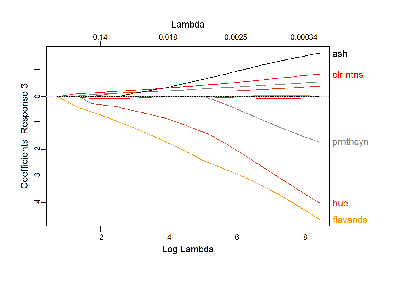
Then, I used 10 fold Cross Validation to find out the best \(\lambda\). You can also see how MSE gets changed based on the change of \(\lambda\).
## 10 fold CV
cvfit=cv.glmnet(x, class, family="multinomial", type.multinomial = "grouped", parallel = TRUE,type.measure = "mse",nfold = 10)
plot(cvfit)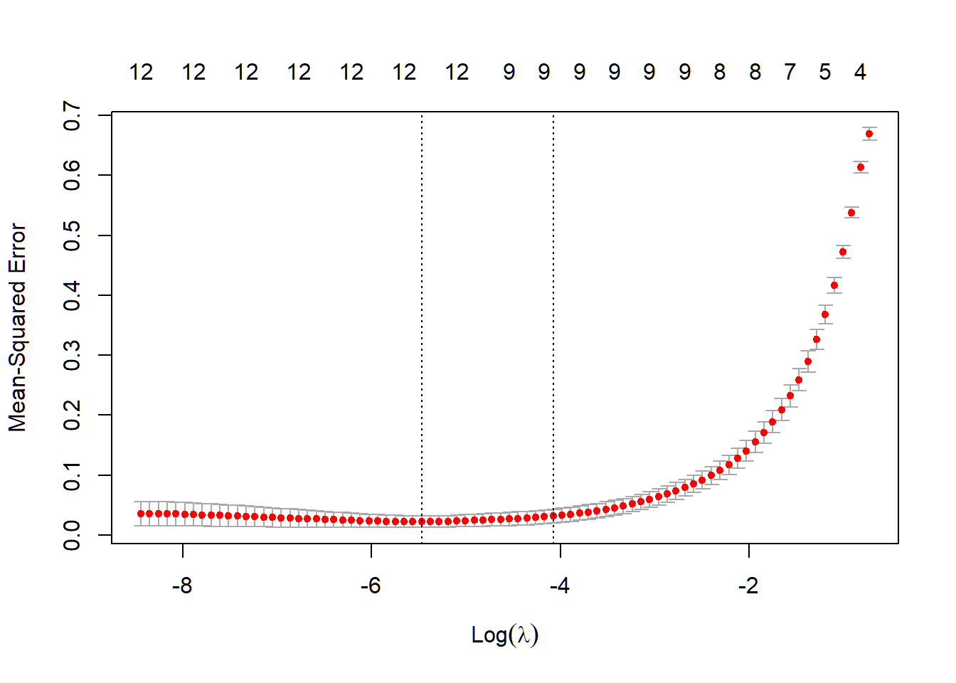
##The best lambda
cvfit$lambda.min
## [1] 0.004214709After I found out the best \(\lambda\), I built up my prediction model based on the training set and \(\lambda\). For testing the performance of this prediction model, I made a confusion matrix and calculate the MSE for testing set.
##making prediction
pred.need=as.matrix(test[,-1])
y_multi_pred_class <- as.numeric(predict(lasso.mod, newx = pred.need, type = "class", s = cvfit$lambda.min))

##making confusion matrix and calculating MSE
xtabs(~ y_multi_pred_class+test$name)
## test$name
## y_multi_pred_class 1 2 3
## 1 26 1 0
## 2 0 28 1
## 3 0 0 151-mean(test$name == y_multi_pred_class)## [1] 0.028169014 ROC curve
For better visualization of the performance of my model, I decided to plot the ROC curve. However, in most situation, the default ROC curve function was built for the two-classes case. Therefore, for three or more classes, I needed to come up with other functions. By using the idea “one vs. all,” which was treating one class as the true class, and treating the rest classes as false classes, I successfully plotted a ROC curve for each class. The original code for for -loop part was from StackExchange. I took the code and modified it to fit my data. For more information, please go to the resource section.
library(ROCR)

lvls = levels(wine$name)
aucs.test=c()

##plotting the layout
plot(x=NA, y=NA, xlim=c(0,1), ylim=c(0,1),
     ylab='True Positive Rate',
     xlab='False Positive Rate',
     bty='n',main="The ROC curve for test data (one vs all)")
color=c("red","green","blue")
legend('bottomright', legend=c("class.1", "class.2","class.3"),
       col=c("red","green","blue"), lty=1, cex=0.8)

##plotting ROC curve for each class
for(type.id in 1:3){
  score =predict(lasso.mod, newx = pred.need, type = "response", s = cvfit$lambda.min)
  actual.class = test[,1] == lvls[type.id ]
  score=data.frame(score)
  pred = prediction(score[,type.id ],actual.class )
  nbperf = performance(pred, "tpr", "fpr")
  roc.x = unlist(nbperf@x.values)
  roc.y = unlist(nbperf@y.values)
  lines(roc.y ~ roc.x, col=color[type.id], lwd=3,lty=1)
  nbauc1 = performance(pred, "auc")
  nbauc1 = unlist(slot(nbauc1, "y.values"))
  aucs.test[type.id ] = nbauc1
}
lines(x=c(0,1), c(0,1))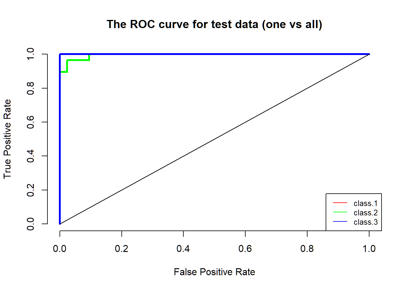
From the graph, you can see the performance of the logistic regression with the lasso penalty is impressive, since all of the ROC curves almost cover the left top corner.
5 Resources
When I was doing this project, I found a lot of useful online sources. Here are some of them:
5.1 ROC Curve
+1. For a better understanding of how R draw ROC curve, I would recommend this video made by Bharatendra Rai. You can learn the ROC curve from the sketch.
https://www.youtube.com/watch?v=ypO1DPEKYFo
+2. I used the followed StackExchange post for building up my ROC curve. The original one was built for dataset iris, and the classifier he used was Naive Bayes https://stats.stackexchange.com/questions/71700/how-to-draw-roc-curve-with-three-response-variable/110550#110550
5.2 About {glmnet}
+1. This is the best website I can find online on how to using {glmnet}. Please have a look.
http://web.stanford.edu/~hastie/glmnet/glmnet_alpha.html#intro