Data project on restaurants' business strategies (Part 1)
1 Data Exploration
The data was collected from Google and Yelp. The samples were from restaurants in 11 metropolitan areas in North America. There were 61 collected variables in total, and this project was mainly interested in 18 of them. In Table 1, you could find more details on the selected 18 variables.
| Variable Name | Variable Type | Unit/ Category | Explanations |
|---|---|---|---|
| Avg_wait_time | Continuous | Hour | The average time on how long costumers spend on waiting for getting dining service |
| Rating | Continuous | Point | The average satisfaction score for each restaurant |
| Num_rating | Continuous | One hundred ratings | The total number of received satisfaction scores by each restaurant |
| Promotion | Continuous | Times | The times of promotion words getting mentioned in the YelpĄŻs comments of each restaurant |
| City | Categorical | Las Vegas, Toronto, Montreal | The city where the restaurant come from |
| Price | Categorical | 1,2,3,4 | The price range which this restaurant belongs to |
| Time | Categorical | Off_weekday,Off_weekend,Peak_weekday,Peak_weekend | The time indicator on peak hour or off-hour of weekday and weekend |
| Arrival_rate | Continuous | Persons per hour | The average arrival rate for different variable time for each restaurant |
| Zip_count | Continuous | Ten restaurants | The number of restaurants which shared the same zip code |
| NoiseLevel | Categorical | Quiet,Average,Loud,Very_loud | The noise level of each restaurant |
| Delivery | Boolean | True,False | The indicator on if the restaurant offers delivery services |
| Reservations | Boolean | True,False | The indicator on if the restaurant offers reservation services |
| TakeOut | Boolean | True,False | The indicator on if the restaurant offers the take out |
| BusinessParking.garage | Boolean | True,False | The indicator on if the restaurant offers the garage parking |
| BusinessParking.lot | Boolean | True,False | The indicator on if the restaurant offers the lot parking |
| BusinessParking.street | Boolean | True,False | The indicator on if the restaurant offers the street parking |
| BusinessParking.valet | Boolean | True,False | The indicator on if the restaurant offers the valet parking |
| BusinessParking.validated | Boolean | True,False | The indicator on if the restaurant offers the validated parking |
You should notice that the promotion words we used were “sale,” “discount,” “coupon,” “promo” and “Groupon”. Also, we removed the extreme case, which had “promotion” to be equal to 0 or larger than 100. For variable “price,” the expenditure for going to the restaurant got increased with “price” increased. Besides, this paper picked three cities, Las Vegas, Montreal and Toronto, which were the top 3 cities that had the most samples in the data. After removing the sample with incomplete information, there were 10093 complete cases left. You could see the total numbers of samples and price distributions in Las Vegas, Montreal, and Toronto in Table 2.
| City | Price 1 | Price 2 | Price 3 | Price 4 | Total |
|---|---|---|---|---|---|
| Las Vegas | 1725 | 2462 | 197 | 61 | 4445 |
| Montreal | 162 | 1187 | 252 | 38 | 1639 |
| Toronto | 554 | 2867 | 505 | 83 | 4009 |
For the distribution of the continuous variables, you could find the information in Figure 1.
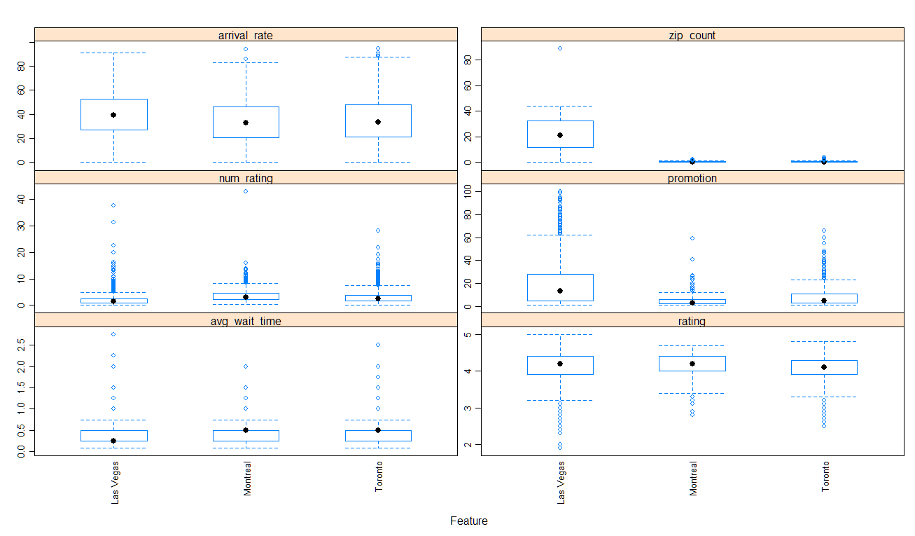
Figure 1.1: The Box plot on arrival_rate, zip_count, num_rating, promotion, avg_wait_time and rating varied by cities
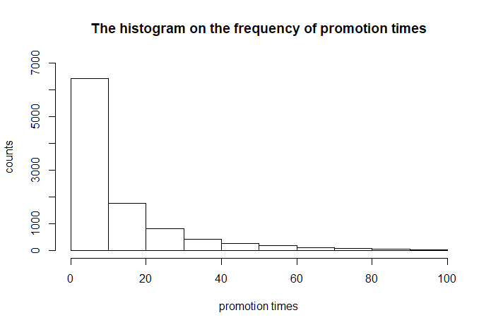
Figure 1.2: The histogram on the frequency of promotion times
2 Methods
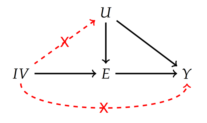
The final explanatory model’s response would be the variable “arrival_rate.” First, we would calculate the residual for an unrefined explanatory model with all 17 variables and their two-way interactions.
Next, for checking if the two-stage least squares (2SLS) was necessary or not, we would calculate the correlation between the residual and each continuous variable. To be more specific, we would calculate correlations between variables and the residual. Some parameters, such as “promotion,” were not normally distributed, which you could observe in the previous part. Therefore, the correlations here were the Kendall’s Rank correlation, instead of the Pearson correlation. Except for variable “price,” The categorical variables here were all exogenous variables. The “price” would be an exogenous and endogenous variable.
If there were some variables, which highly correlated with the residual, we would use the 2sls and build the first stage linear regression model on those endogenous variables with some instrument variables. For the model selection, we would use the backward model selection to choose the final explanatory linear regression model from the full model with 17 parameters and all their two-way interactions by comparing their AIC. If there were not such parameters, that correlated with the residual, we would directly jump to the model selection part.
3 R Coding
Notice that since the data file is very large, we won’t actually run the code on the web. First, let’s check the correlation between the residual and each variable. From the Figure 3, you could see the correlation between the residual and each continuous variable in the red ellipse.
library(readr)
library(stringi)
library(stringr)
library(tidyr)##for function unite
library(corrplot)##for function corrplot

test<- read_csv("D:/research/final full data/longWithZip_time.csv")
table(test$city)

##pick Las Vegas, Toronto and Montral's restaurants and combine them to get our final dataset
lv=subset(test,test$city=="Las Vegas")
to=subset(test,test$city=="Toronto")
mo=subset(test,test$city=="Montral")
sub=rbind(lv,to,mo)

##keep interested parameters
testcity=data.frame(sub$avg_wait_time,sub$rating,sub$rating_n,sub$promotion,sub$city,
                    sub$attributes_RestaurantsPriceRange2,sub$arrival,sub$hour,
                    sub$day,sub$Freq,sub[,c(40,43,46,48,12:16)])

##keep the restaurant with full info
testcity=testcity[complete.cases(testcity),]

##change the parameters' names

names(testcity) = c('avg_wait_time'
                    ,'rating'
                    ,'num_rating'
                    ,'promotion'
                    ,'city'
                    ,'price'
                    ,'arrival_rate'
                    ,'hour'
                    ,'day'
                    ,'zip_count'
                    ,'NoiseLevel'
                    ,'Delivery'
                    ,'Reservations'
                    ,'TakeOut'
                    ,'BusinessParking.garage'
                    ,'BusinessParking.lot'
                    ,'BusinessParking.street'
                    ,'BusinessParking.valet'
                    ,'BusinessParking.validated'

)


##combine param: hour and day to get a new param: time
testcity=unite(testcity,time, c(hour,day), remove=TRUE)

##change data scale
alter.data=subset(testcity,testcity$promotion!=0)
alter.data=alter.data[which( alter.data$promotion<=100),]
alter.data$avg_wait_time=alter.data$avg_wait_time/60
alter.data$num_rating=alter.data$num_rating/100
alter.data$zip_count=alter.data$zip_count/10

##Get kendall correlation plot on correlation between residual and the rest numerical params
y=lm(arrival_rate~.*.,data=alter.data)
new.data=data.frame(resid((y)),alter.data[,-c(5,8)])
corrplot.mixed(cor(new.data,method="kendall"),lower.col = "black", number.cex = .9,tl.col = "black")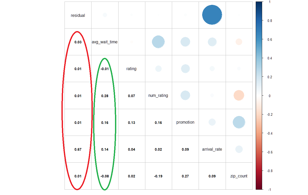
Figure 3.1: The correlation plot between the residual and each continuous variable
As you can see, except the response variable, the variable “avg_wait_time” had the highest correlation with the residual. It mean we could consider of the 2sls, and build first stage linear regression model with the response “avg_wait_time.” For the choice of instrument variables, in the green ellipse, you could notice that “num_rating,” “promotion,” and “zip_count” were highly correlated with “avg_wait_time.” Based on those observations, we built the first stage linear regression model, whose response was variable “avg_waiting_time”, and the instrument variables were “num_rating”, “price”, “promotion” and “zip_count”.
##predict the avg_wait_time
alter.data$price=as.factor(alter.data$price)
m1=lm(avg_wait_time~num_rating+price+promotion+zip_count,data=alter.data)
summary(m1)
predict.average.time=fitted.values(m1)
Then, for the second stage:
##remove awg_waiting_time, num_rating and zip_count, add predict.average.time
new=data.frame(data3[,-c(1,3,9)],predict.average.time)
new$time=as.factor(new$time)

## second stage(using anova to find the best model)
m3=lm(new$arrival_rate~.*.,data=new)
n=step(m3)
summary(n)
4 Results
This data project is a part of paper All Gains, No Pain? Optimal Promotion Strategies with Delay Sensitive Customers, written by Prof. Guangwen Kong. For the final result, please check this paper.