Data project on restaurants' business strategies (Part 2)

1 Introduction
In March 2018, I joined in Prof. Kong’s data research project for validating her theoretical model. The used dataset was generated from Yelp dataset (https://www.yelp.com/dataset/challenge) and Google Map, which offered a lot of time-related information. In total, the final dataset had about 2 GB. There were nearly hundreds of parameters in this file. The file was also wroten in JSON. Because I have never had any experience in dealing with large JSON file before, I decided to covert the data into a CSV file, which I was more familiar with. After converting, unsurprisingly, the file’s size got doubled. The file became even more impossible for R Studio and Excel to open in my laptop. Therefore, after googling around, I decided to use Delimit (http://www.delimitware.com/), which was a software can quickly open and modify a large CSV file. By using this software, I kept around 80 interested parameters and divided the data into seven smaller CSV files, which each one can be opened easily by R Studio.
2 Digging for the information
##1: Finding promotion, waiting time, address and zip_count
First, Let’s look at the some original parameters.

Figure 2.1: of Parameters(Part 1)
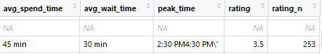
Figure 2.2: Part of Parameters(Part 2)
For collecting promotion information, we decided to search keywords, such as “sale”,“discount”,“coupon”,“promotion”,“groupon”, and “offer”, from Yelp users’ reviews. In this dataset, rows were differed by Yelp users’ reviews and followed users’ info. It means each restaurant could have several rows in this dataset. Our plan was counting the appearances of the keywords from each user’s review. Then, we could determine if the user got promotion based on if there is a keyword showed up in his/her review. Eventually, we could know how often each restaurant does promotion later. Also, we could keep the data varied by restaurants, insted of varied by Yelp’s users.
library(readr)
X1 <- read_csv("D:/research/final full data/excel/7.csv")


## count promotion information
keywords<-c("sale","discount","coupon","promotion","groupon", "offer")

##change the text to lower case
x=sapply(X1$review_text, tolower)
##use grepl to count the words
m = sapply(keywords, grepl,x)
m=m*1
promo.info=transform(m, sum=rowSums(m))
##determine if the user had a promo or not
promo.info$sum=1*(promo.info$sum>0)
datapart=cbind(X1,promo.info)
datapart=as.data.frame(datapart)

##remove temporary and unimportant columns
cols.dont.want <- c("cool","date","funny","review_text","review_id","review_star","useful","user_id","sale","discount","coupon","promotion","groupon", "offer")
datapart <- datapart[, ! names(datapart) %in% cols.dont.want, drop = F]

## get reduced store list
w=tapply(datapart$sum,datapart$business_id,sum)
w=data.frame(w)
library(data.table)
w=setDT(w, keep.rownames = TRUE)[]
names(w)[names(w)=="rn"]<-"business_id"
names(w)[names(w)=="w"]<-"promotion"

##Back to the dataset combine it with the promotion info by unique business id
deduped.data <- unique( datapart[,1:69])
deduped.data=data.frame(deduped.data)
merge.data=merge(w,deduped.data,by="business_id")
merge.data=merge.data[complete.cases(merge.data[ ,1:2]),]
merge.data=merge.data[complete.cases(merge.data$address)]
Then, we changed avg_waiting_time (see prvious Figure 2) from text to numeric. Becasue we could have “1h25min”, the situation got a little different from data type changing.
##change average waiting time
time=c("1 hour","10 min", "15 min", "1h 15m", "1h 30m","1h 45m","2 hours","20 min","25 min","2h 15m","2h 30m","2h 45m","3 hours","30 min","45 min","5 min")
t=c(60,10,15,75,90,105,120,20,25,135,150,165,180,30,45,5)
for(i in 1:16){
  merge.data$avg_wait_time[merge.data$avg_wait_time==time[i]]<-t[i]
}
merge.data$avg_wait_time=as.numeric(merge.data$avg_wait_time)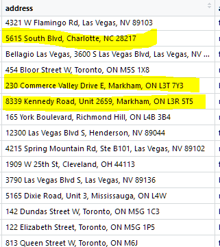
Figure 2.3: Part of Parameters(Part 3)
As you can see the hightlight part, because of having Canandian cities and American cities, the data address was not in the united form. Since we only wanted to keep cities’ name and zip for zip_count, we needed to do some extra work. Here, I used package stringi and stringr.
library(stringi)
library(stringr)

##cince city is in the last second, so I reverse the text
merge.data$address=stri_reverse(merge.data$address)

##spilit the text by comma
x=str_split_fixed(merge.data$address, ",",3)

##Take out the "city"
x=data.frame(x)
merge.data=data.frame(merge.data,x)
names(merge.data)[names(merge.data)=="X2"]<-"city"
names(merge.data)[names(merge.data)=="X1"]<-"zip"
merge.data$city=stri_reverse(merge.data$city)
merge.data$zip=stri_reverse(merge.data$zip)

##throw away unwanted info
cols.dont.want <- c("address","X3")

##combine and save the data
merge.data <- merge.data[, ! names(merge.data) %in% cols.dont.want, drop = F]
write.csv(merge.data,"D:/research/final full data/data7.csv",row.names = F)
Next, let’s combine seven datasets to get samller complete data set.
X1 <- read_csv("D:/research/final full data/data1.csv")
X2 <- read_csv("D:/research/final full data/data2.csv")
X3 <- read_csv("D:/research/final full data/data3.csv")
X4 <- read_csv("D:/research/final full data/data4.csv")
X5 <- read_csv("D:/research/final full data/data5.csv")
X6 <- read_csv("D:/research/final full data/data6.csv")
X7 <- read_csv("D:/research/final full data/data7.csv")


library(reshape)
library(reshape2)
list_df <- list(X1,X2,X3,X4,X5,X6,X7)
merged_df <- merge_all(list_df)
merged_df$index <- as.numeric(row.names(merged_df))
merged_df=merged_df[order(merged_df$index), ]
cols.dont.want <- c("index")
merged_df <- merged_df[, ! names(merged_df) %in% cols.dont.want, drop = F]
merged_df=unique(merged_df)

##dor remove the repeated restaurant in different dataset
w=tapply(merged_df$promotion,merged_df$business_id,sum)
w=data.frame(w)
library(data.table)
w=setDT(w, keep.rownames = TRUE)[]
names(w)[names(w)=="rn"]<-"business_id"
names(w)[names(w)=="w"]<-"promotion"

cols.dont.want <- c("promotion")
merged_df <- merged_df[, ! names(merged_df) %in% cols.dont.want, drop = F]
final <- unique(merged_df)
final=merge(w,final,by="business_id")

##counting how many retaurants share the same zip code
final$zip=as.factor(final$zip)
t=as.data.frame(table(final$zip))
names(t)[names(t)=="Var1"]<-"zip"
address.final=merge(final,t,by="zip")


write.csv(address.final,"D:/research/final full data/final.csv",row.names = F)
2.1 2: About peak time and arrival rate
I believed this was one of the most challenging parts for this project. The arrival rate was defined as the average arrival rate for a different time, such as Off_weekday, Off_weekend, Peak_weekday, and Peak_weekend, for each restaurant. From the provided data (see Figure 1 & 2), we had an arrival count for each hour of each day, and we also had a peak_time(Figure 2). For the restaurant, which didn’t have a peak hour range, we set a peak hour. For the restaurant, which didn’t have arrival count information, we discarded that restaurant.Here is the step:
library(readr)
library(stringi)
library(stringr)
final <- read_csv("D:/research/final full data/final.csv")

##get peak hour
###split peak_time into time.1(start) and time.2(end) by "M"
time=str_split_fixed(final$peak_time, "M",2)
time=data.frame(time)
##split time.1(start) to get time and info on PM/AM
time.1=str_split_fixed(time$X1, " ",2)
time.1=data.frame(time.1)
##we only want whole time, not things after ":""
peak=stri_reverse(gsub("^.*?:",":",stri_reverse(time.1$X1)))##reverse for removing things after ":"
time.1=data.frame(time.1,peak)
time.1$peak=gsub(":"," ",time.1$peak)
cols.dont.want <- "X1" # if you want to remove multiple columns
time.1 <- time.1[, ! names(time.1) %in% cols.dont.want, drop = F]
names(time.1)[names(time.1)=="X2"]<-"T1"

##For time.2(end), we need to have some extra step on removing"\"
#split time.1(end) to get time
time.2=str_split_fixed(time$X2, " ",2)
time.2=data.frame(time.2)
end=stri_reverse(gsub("^.*?:",":",stri_reverse(time.2$X1)))
time.2=data.frame(time.2,end)
time.2$end=gsub(":"," ",time.2$end)
##get info on PM/AM
zone=str_split_fixed(time.2$X2, "M",2)
zone=data.frame(zone)
cols.dont.want <- c("X1", "X2") # if you want to remove multiple columns
time.2 <- time.2[, ! names(time.2) %in% cols.dont.want, drop = F]
time.2=data.frame(zone$X1,time.2)
names(time.2)[names(time.2)=="zone.X1"]<-"T2"

##get peak time
final.time=data.frame(time.1,time.2)

## adjust time into 24 hours based on PM/AM by adding 12
for( i in 1:54635){
  if (final.time$T1[i]=="P"){
    final.time$peak[i]=as.numeric(final.time$peak[i])+12
  }
}

for( i in 1:54635){
  if (final.time$T2[i]=="P"){
    final.time$end[i]=as.numeric(final.time$end[i])+12
  }
}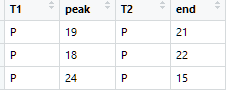
Figure 2.4: for peak time range
After figuring out peak hour range, it is time to get arrival rate. Since there are 7 days per week, we take Monday as an example. Also, notice few things: First, peak_hour was set same though Mon to Sun. Second, for off-hour, we mean hours whith arrival rate =0 and are not in peak hour range
################Monday

##since the arrival rate was record as [0,1,1,1,1...], we split the array into 24 conlumns
monday=str_split_fixed(final$monday, ",",24)
monday=data.frame(monday)

##remove [ ]
monday$X24=gsub("]"," ",monday$X24)
monday$X1=gsub("\\["," ",monday$X1)
monday$X1=gsub("]"," ",monday$X1)

for(i in 1:24){
  monday[,i]=as.numeric(as.character((monday[,i])))
}
monday=data.frame(monday,final.time)
monday$peak=as.numeric(monday$peak)
monday$end=as.numeric(monday$end)
monday[is.na(monday)]<-0
c=c(as.numeric(monday[15,20:22]))
v=mean(c)
f.t=data.frame(peak1.h=c(rep(0,times=54635)),off1.h=c(rep(0,times=54635)))


for(i in 1:54635){
  ##if there is no info on peak hour range
  if(monday$peak[i]==0&&monday$end[i]==0){
    p.1=as.numeric(monday[i,11:14])
    p.2=as.numeric(monday[i,17:20])
    p.h=c(p.1,p.2)
    ##for off hour, remove closed hour, which is the hour whith arrival rate =0and is not in peak hour range
    rest=as.numeric(monday[i,-c(11:14,17:20,25:28)])
    p.h=p.h[p.h!="0"]
    rest=rest[rest!="0"]
    f.t$peak1.h[i]=mean(p.h)
    f.t$off1.h[i]=mean(rest)
  }
  ## if peak hour end in the same day
  else if (monday$peak[i]<=monday$end[i]){
    f.t$peak1.h[i]=mean(as.numeric(monday[i,monday$peak[i]:monday$end[i]]))
    rest=as.numeric(monday[i,-c(monday$peak[i]:monday$end[i],25:28)])
    rest=rest[rest!="0"]
    f.t$off1.h[i]=mean(rest)
  }

  ##if the peak hour lasted for two days
  else if(monday$peak[i]>monday$end[i]){
    p=as.numeric(monday[i,monday$peak[i]:24])
    q=as.numeric(monday[i,1:monday$end[i]])
    p.h=c(p,q)
    rest=as.numeric(monday[i,-c(monday$peak[i]:24,1:monday$end[i],25:28)])
    rest=rest[rest!="0"]
    f.t$peak1.h[i]=mean(p.h)
    f.t$off1.h[i]=mean(rest)
  }

}
final=data.frame(final,f.t)


###############calculating Off_weekday, Off_weekend, Peak_weekday, and Peak_weekend

cols.dont.want <- c("friday","monday","tuesday","sunday","saturday","wednesday","thursday","peak_time") # if you want to remove multiple columns
final.1 <- final[, ! names(final) %in% cols.dont.want, drop = F]

Data=data.frame(final.1,final.time)##final.time for peak_hour range
peak_weekday=c(rep(0,times=54635))
off_weekday=c(rep(0,times=54635))
peak_weekend=c(rep(0,times=54635))
off_weekend=c(rep(0,times=54635))

for(i in 1:54635){
peak_weekday[i]=mean(c(Data$peak5.h[i],Data$peak1.h[i],Data$peak2.h[i],Data$peak3.h[i],Data$peak4.h[i]))
off_weekday[i]=mean(c(Data$off5.h[i],Data$off1.h[i],Data$off2.h[i],Data$off3.h[i],Data$off4.h[i]))
peak_weekend[i]=mean(c(Data$peak6.h[i],Data$peak7.h[i]))
off_weekend[i]=mean(c(Data$off6.h[i],Data$off7.h[i]))
}

data=data.frame(Data,peak_weekday,peak_weekend,off_weekday,off_weekend)
write.csv(data,"D:/research/final full data/complete_time.csv",row.names = F)
3 Thoughts
Here is the final data sample:
Figure 3.1: Part of final data sample
For this project, I got to know a lot new packages. In the end, I want to say that observation of data is really important; otherwise, you may struggle a lot and get nothing from it.