Introduction on Multi-stage Robust Optimization
1 Introduction
Multistage robust optimization is focused on the worst-case optimization problem affected by uncertainty under a dynamic setting. Unlike static robust optimization problems, which all decisions are implemented simultaneously and before any uncertainty is realized, the multistage robust optimization, however, includes some adjustable decisions, which depend on the revealed data before the decisions are made. Therefore, multistage robust optimization is also called adaptive robust multistage optimization or adjustable robust multistage optimization. Although robust optimization has already been discussed for decades, multistage robust optimization is a relatively new topic. In 2002, A. Ben-Tal, A. Goryashko, and A. Nemirovski were the first to discuss robust multistage decision problems, opening the field to numerous other papers either dealing with theoretical concepts or applying the framework to practical problems, such as inventory management, energy generation and distribution, portfolio management, facility location and transportation, dynamic pricing and so on.
2 Decisions Types
Based on the choice of whether people allow their decisions to be dependent on the revealed information or not, there can be two kinds of decisions.
Here-and-now decision: Those decisions should be made as a result of solving the problem before the actual data “reveals itself” and as such should be independent of the actual values of the data.
Wait-and-see decisions: Those decisions could be made after the controlled system “starts to live,” at time instants when part (or all) of the true data is revealed. It is fully legitimate to allow for these decisions to depend on the part of the data that indeed “reveals itself” before the decision should be made.
3 General Formulation
For a better understanding of the formulation of adjusted robust multistage optimization, let’s consider a general-type uncertain optimization problem-a collection
\[ p=\{min_{x}\{f(x,\xi):F(x,\xi)\in K\}:\xi\in \Xi\}.............(1)\]
of instances - optimization problems of the form
$ min_{x}{f(x,):F(x,)K}$
where \(x \in R^n\) is the decision vector, \(\xi\in R^L\) represents the uncertain data, the real-valued function \(f(x;\xi)\) is the objective, and the vector-valued function \(F(x;\xi)\) takes values in \(R^m\) along with a set \(K\subset R^m\) specify the constraints; finally, \(\Xi\subset R^L\) is the uncertainty set.
The Robust Counterpart (RC) of uncertain problem (1) is defined as \[ min_{x,t}\{t:\forall \xi \in \Xi: f(x,\xi)\leqslant t,F(x,\xi)\in K\}.............(2)\] Therefore, all the decision variables x are here-and-now decisions.
Now, we want to adjust the robust counterpart so that we can corporate the wait-and-see decisions into the decision making process.
First, let’s define \(\forall j \leqslant n\): \[ x_j=X_j(P_j \xi)........(3)\] where \(P_j\) are given in advance matrices specifying the “information base” of the decisions \(x_j\). In other words, \(P_j\)’s value will decide how much portion of the true data that \(x_j\) can depend on. \(X_j()\) are called decision rules; these rules can in principle be arbitrary functions on the corresponding vector spaces.
The Adjusted Robust Counterpart (ARC) of uncertain problem (1) is defined as \[min_{t,\{X_j()\}^n_{j=1}}\{t:\forall \xi \in \Xi: f(X(\xi),\xi)\leqslant t,F(X(\xi),\xi)\in K\}\]
\[X(\xi)=[X_j(P_j \xi)], \forall j\in n........(4)\] by replacing the the decision variables \(x_j\) in (2) with function (3). Note that the ARC is an extension of the RC; the latter is a case of the former corresponding to the case of trivial information base in which all matrices \(P_j\) are zero, so that \(x_j\) are here-and-now decision.
4 Policies Choice
From the computational viewpoint, solving a robust multi-stage linear programming model is NP-hard[4]. The reason comes from the fact that the ARC is typically severely computationally intractable. The equation (4) is an infinite-dimensional problem, where one wants to optimize over functions -decision rules- rather than vectors, and these functions, in general, depend on many real variables. Seemingly the only option here is sticking to a chosen in advance parametric family of decision rules, like piece-wise constant/linear/quadratic functions of \(P_j(\xi)\) with simple domains of the pieces. With this approach, a candidate decision rule is identified by the vector of values of the associated parameters, and the ARC becomes a finite-dimensional problem, the parameters being our new decision variables. This approach is indeed possible and in fact will be the focus of what follows.
4.1 Static Policies
The simplest type of policy to consider is a static one, whereby all future decisions are constant and independent of the intermediate observations. Such policies do not increase the underlying complexity of the decision problem, and often they result in tractable robust counterparts. For instance, this kind of policy can be optimal for LPs with row-wise uncertainty. Here is an example \[P=\{min_x\{c^T_\xi x+d_\xi:a^T_{i\xi}x\leq b_{i\xi},i=1,...,m\}:\xi\in \Xi\}\]
where the uncertainty vector can be partitioned into \(J + 1\) blocks. Also, its objective depend solely on \(\xi_0\in \Xi_0\), and the data in the jth constraint depend solely on \(\xi_j\in \Xi_j\).
4.2 Affine Decision Rules
Consider an affinely perturbed uncertain conic problem: \[ C=\{min_{x\in R^n}\{c^T_{\xi}x+d_{\xi}:A_{\xi}x+b_{\xi}\in K: \xi \in \Xi\}...........(5)\]
where $c_{} ; d_{} ;A_{} ; b_{} $ are affine in \(\xi\), K is a cone, which is the direct product of nonnegative rays, and \(\Xi\) is a convex compact uncertainty set defined as following
\[\xi=\{\xi\in R^L: \exists u : \bf{P}(\xi,u)\succeq 0\}\]
where P is affine in \([\xi; u]\). Assume that along with the problem, we are given an information base \(\{P_j\}^n_{j=1}\)for it; here \(P_j\) are \(m_j*n\) matrices.Then we need to use affine decision rules to approximate the ARC of the problem.
Affine decision rules will have the following structure: \[x_j=X_j(P_j\xi)=p_j+q^T_jP_j\xi,j=1,...,n.............(6)\]
Hence,Affinely Adjustable Robust Counterpart (AARC), which is the resulting restricted version of the ARC of (5), will be \[min_{t,\{p_j,q_j\}^n_{j=1}} \{\{ t: \sum_{j=1}^n c^j_\xi[ p_j+q_j^T P_j \xi ]+d_\xi-t \leq 0, \sum_{j=1}^n A^j_\xi[ p_j+q_j^T P_j\xi ]+b_\xi\in K \}\forall \xi\in \Xi\} \]
where where \(c^j_{\xi}\)is j-th entry in \(c_\xi\) , and \(A^j_\xi\) is j-th column of \(A_\xi\) . Note that the variables in this problem are t and the coefficients \(p_j,q_j\) of the affine decision rules (6). As such, these variables do not specify uniquely the actual decisions \(x_j\); these decisions are uniquely defined by these coefficients and the corresponding portions \(P_j\xi\) of the true data once revealed.
For illustration, you can take a look on section 5.3.4 on one of the reference books Robust Optimization. That is a example on applying AARC to a simple multi-product multi-period inventory model.
4.3 Piecewise Affine Decisions Rules
It is to be expected that in the general case, applying affine decision rules will generate suboptimal policies compared to fully adjustable ones. Thus, one might be tempted to investigate whether tighter conservative approximations can be obtained by employing more sophisticated (yet tractable) decision rules, in particular, nonlinear ones. Below are some examples of how this can be achieved by taking piecewise affine decision rules. === K Adaptability=== Consider now a multi-stage optimization where the future stage decisions are subject to integer constraints. The framework introduced above cannot address such a setup, since the later stage policies, \(X_j(P_j\xi)\), are necessarily continuous functions of the uncertainty. The setting of K Adaptability is to deal with the situation mentioned in the previous section. It is introduced here: Finite Adaptability in Multistage Linear Optimization
Here is an example. Let’s start with a simple case, i.e., the two-stage Robust optimization. Suppose the second -stage variables,\(x_2=X_2(P_2\xi)\), are piecewise constant functions of the uncertainty, with k pieces. Due to the inherent finiteness of the framework, the resulting formulation can accommodate discrete variables. In addition, the level of adaptability can be adjusted by changing the number of pieces in the piecewise constant second stage variables. Consider a two-stage problem of the form
\[min: c^T x_1+d^T x_2 \] \[s.t: A_1(\xi)+A_2(\xi)x_2\geq b, \forall \xi\in \Xi\] \[x_1\in \chi_1,x_2\in \chi_2\] where \(\chi_2\) may contain integrality constraints. In the k adaptability framework, with k-piecewise constant second stage variables, this becomes
\[Adapt_k(\xi)= min_{\Xi=\Xi_1\cup...\cup \Xi_k} \left \{ min: c^T x_1+max\{d^T x_2 ^{(1)},...,d^T x_2 ^{(k)}\}\\ s.t: A_1(\xi)+A_2(\xi)x_2 ^{(1)}\geq b, \forall \xi\in \Xi_1\\ .\\ .\\ .\\ A_1(\xi)+A_2(\xi)x_2 ^{(k)}\geq b, \forall \xi\in \Xi_k\\ x_1\in \chi_1,x_2^{(j)}\in \chi_2 \right \}\] If the partition of the uncertainty set, \(\Xi=\Xi_1\cup...\cup \Xi_k\) is fixed, then the resulting problem retains the structure of the original nominal problem, and the number of second stage variables grows by a factor of k. Furthermore, the static problem (i.e., with no adaptability) corresponds to the case k = 1, and hence if this is feasible, then the k-adaptable problem is feasible for any k. This allows the decision-maker to choose the appropriate level of adaptability. This flexibility may be particularly crucial for substantial scale problems, where the nominal formulation is already on the border of what is currently tractable.
The complexity of K adaptability is in finding a suitable partition of the uncertainty. In general, computing the optimal partition even into two regions is NP-hard. However, we also have the following positive complexity result. It says that if any one of the three quantities:(a) Dimension of the uncertainty; (b) Dimension of the decision-space; and (c ) Number of uncertain constraints, is small, then computing the optimal 2-piecewise constant second stage policy can be done efficiently.
4.4 Other Piecewise Decision Rule Design
Although decision rules have been established as the preferred solution method for addressing multistage adaptive optimization problems. However, previously mentioned methods cannot efficiently design binary decision rules for multistage problems with a large number of stages, and most of those decision rules are constrained by their a prior design. In 2014, Dimitris Bertsimas and Angelos Georghiou proposed a new designing way to address those problems. In their papers, they derive the structure for optimal decision rules involving continuous and binary variables as piecewise linear and piecewise constant functions, respectively. Then, they propose a methodology for the optimal design of such decision rules with finite pieces and solve the problem using mixed integer optimization. For more details, You can find paper here
5 An Example on Inventory Management
Here, this example will show you how to apply ARC framework to formulate a problem. Let’s consider a simple inventory problem in which a retailer needs to order some goods to satisfy demand from his customers while incurring the lowest total cost, which is the sum of the cost for ordering \((c_t)\), holding\((h_t)\), and backlogging \((b_t)\) over a finite time horizon. First, we can formulate a deterministic model where implementable and auxiliary decisions can be identifieded: \[min_{x_t,S_t^+,S_t^-} \sum^T_{t=1}(c_t x_t+h_t s_t^+ +b_t s_t^-)\] \[s.t. s^+_t\geq 0, s^-_t \geq 0, \forall t\] \[s^+_t \geq y_1+\sum^t_{t'=1} x_{t'}-d_{t'} ,\forall t \] \[s^-_t \geq -y_1+ \sum^t_{t'=1}d_{t'}-x_{t'},\forall t,\] \[0\leq x_t\leq M_t,\forall t\] Here, \(x_t\) is number of goods ordered at time t and received at t+1; \(y_t\) is number of goods in stock at beginning of time t; * \(d_t\) is demand between time t and t+1 * \(M_t\) is max order size * \(s_t^+\) is amount of goods held in storage during stage t * \(s_t^-\) is amount of backlogged customer demands during stage t
Then, one might consider that at each point of time, the inventory manager can observe all of the prior demand
before placing an order for the next stage. This could apply, for instance, to the case when
the entire unmet demand from customers is backlogged, so censoring of observations never
arises. Then, the sequence of decision variables and observations can be defined as follows
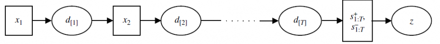
From the figure [5], it is clear that \(s^+_t\) and \(s^-_t\) are auxiliary variables that are adjustable with respect to the full uncertainty vector \(d_{[T]} =d\). Once \(d_{[T]}\) is revealed, the uncertainty can be considered reduced to zero. Hence, we can reformulate the previous problem by using a multistage ARC model: \[min_{x_1,\{x_t()\}^T_{t=2},\{S_t^+(),S_t^-()\}^T_{t=1}} \sum^T_{d\in U}(c_t x_t(d_{[t-1]})+h_t s_t^+(d) +b_t s_t^-(d))\] \[s.t. s^+_t(d)\geq 0, s^-_t (d)\geq 0, \forall t,\forall d\in U\] \[s^+_t(d) \geq y_1+\sum^t_{t'=1} x_{t'}(d_{[t-1]})-d_{t'} ,\forall t,\forall d\in U \] \[s^-_t (d)\geq -y_1+ \sum^t_{t'=1}d_{t'}-x_{t'}(d_{[t-1]}),\forall t,\forall d\in U\] \[0\leq x_t(d_{[t-1]})\leq M_t,\forall t,\forall d\in U\] where \(U \subseteq R^T\)
For more about stochastic optimization, go check: here
6 Reference
[1] Bertsimas, Dimitris; Brown, David; Caramanis, Constantine, “Theorey and applications of Robust Optimization,” Oct 2010. [Online]. Available: {https://ui.adsabs.harvard.edu/abs/2010arXiv1010.5445B.
[2] W. S. Choe, “Adaptive robust optimization,” 2015. [Online]. Available: https://optimization.mccormick.northwestern.edu/index.php/Adaptive_robust_optimization. [Accessed 13 April 2019].
[3] C. Gounaris, “Modern Robust Optimization: Opportunities for Enterprise-Wide Optimization,” Dept. of Chemical Engineering and Center for Advanced Process Decision-making Carnegie Mellon University, 7 September 2017. [Online]. Available: http://egon.cheme.cmu.edu/ewo/docs/EWO_Seminar_09_07_2017.pdf. [Accessed 13 April 2019].
[4] A.Ben-Tal, L. El Ghaoui and A. Nemirovski, Robust Optimization, Princeton University Press, 2009.
[5] Erick DelageDan A. Iancu. Robust Multistage Decision Making. In INFORMS TutORials in Operations Research. Published online: 26 Oct 2015; 20-46. https://doi.org/10.1287/educ.2015.0139