Animation meets Gradient Decent
1 Introduction
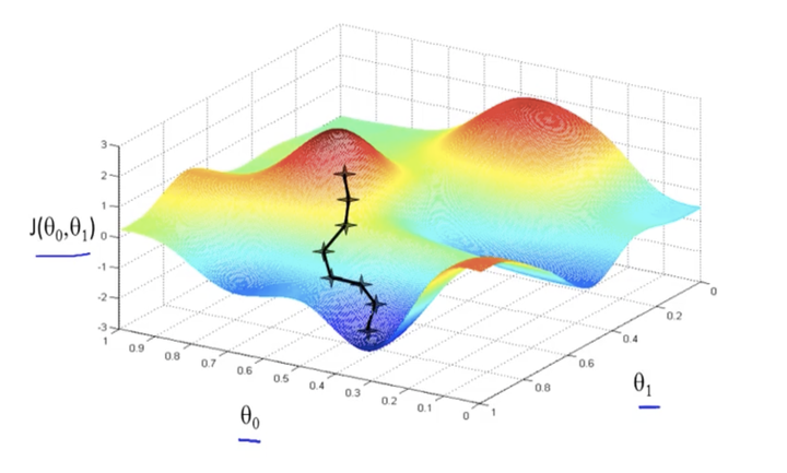
Gradient descent is an optimization algorithm used to minimize some function by iteratively moving in the direction of steepest descent as defined by the negative of the gradient. In machine learning, we use gradient descent to update the parameters of our model. Parameters refer to coefficients in Linear Regression and weights in neural networks.
2 Algorithm
Here is the algorithm:
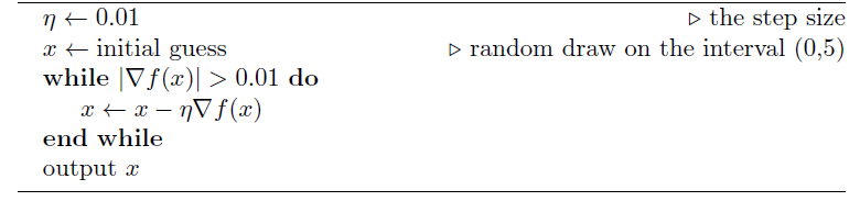
3 Example
3.1 1D case
First, let’s start with a simple case. Suppose we need to find \(x\) that mimize \[f(x)=1+(x-3)^{2}\] by using the gradient decent which described in the algorithm
gradient_descent = function(step_size,initial_guess){
  x = initial_guess
  d_fx=10

  while(abs(d_fx)>0.01){
    d_fx = 2*(x-3)
    x = x-step_size*d_fx

  }

  return(x)
}
Now, let’s visulize the result by checking if we find the minimum point or not. You should be able to see the red dots(the found solution) appeared at the bottom of the function curve
x = gradient_descent(0.01,0)
x
## [1] 2.995136##Check
t= seq(0,5,by = 0.01)
y = 1+(t-3)^2
plot(t,y)
points(x,1+(x-3)^2,col='red',pch=23,lwd=6)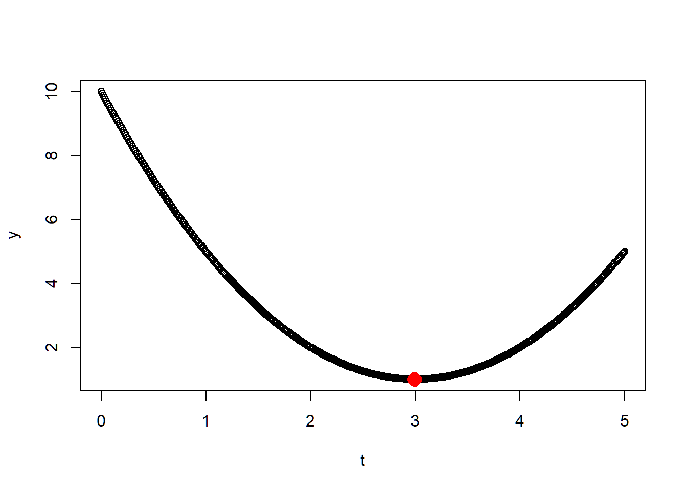
Yes! We made it. Now, let’s try the case in 2D.
3.2 2D case
Suppose we need to find \(x = [x_1,x_2]\) that mimize
\[f\left(x_{1}, x_{2}\right)=1+\left(x_{1}-3\right)^{2}+\left(x_{2}-2\right)^{2}\]
by using the gradient decent which described in the algorithm
gradient_descent = function(step_size,initial_guess){
  x = initial_guess
  d_fx= rep(10,length(initial_guess))
  N =10000
  trace <- vector("list", N)
  i = 1
  while(max(abs(d_fx))>0.01){
    d_fx[1] = 2*(x[1]-3)
    d_fx[2] = 2*(x[2]-2)
    x = x-step_size*d_fx
    trace[[i]] <- x
    i <- i + 1

  }
  result = list("answer"=x,"trace"=Filter(Negate(is.null), trace) )
  return(result)
}
library(data.table)
x = gradient_descent(0.01,c(-10,-10))
trace_loc = transpose(as.data.frame(x$trace))
colnames(trace_loc )=c("t1","t2")
trace_loc$z = 1+(trace_loc$t1-3)^2+(trace_loc$t2-2)^2
trace_loc$episode = seq(1,length(trace_loc$z),1)
3.3 Using plotly to make an animation
Plotly’s R graphing library makes interactive, publication-quality graphs. For this 2D case, we can make an animation to visualize the trajectory of the decent by using Plotly.
##Check
library("plotly")
library(reshape2)
library(rlist)
t1= seq(-10,10,by = 0.1)
t2= seq(-10,10,by =0.1)
z =outer(1+(t1-3)^2,(t2-2)^2,`+`)
rownames(z) <- seq(-10,10,by =0.1)
colnames(z) <-seq(-10,10,by =0.1)
matrix=melt(z)
data=setNames(matrix, c("t1", "t2", "VALUE"))

fig = plot_ly(x = ~data$t1, y = ~data$t2, z = ~data$VALUE,type = 'scatter3d',mode ='lines',
              line = list(color = '#1f77b4', width = 1.5))
fig <- fig %>% add_trace( x = ~trace_loc$t1, y = ~trace_loc$t2, z = ~trace_loc$z,
                           type = 'scatter3d',mode = 'lines',
                           line = list(color = 'yellow', width = 10))
fig <- fig %>% add_markers( x = ~trace_loc$t1, y = ~trace_loc$t2, z = ~trace_loc$z,
                          frame = ~trace_loc$episode, type = 'scatter3d',mode = 'markers',
                          showlegend = F,color = 'green')


fig
4 Reference
- For using
Plotlyto make animation, I used the tutorial from here: https://plotly.com/r/animations/